1.7 Economic Transformation of India Through Railways in the Pre-Independence Era

The advent of railways in pre-independent India marked a pivotal moment in the subcontinent’s economic history. Conceived and developed under British colonial rule, this vast network of iron tracks profoundly reshaped India’s economic landscape, impacting trade, agriculture, industry, and social structures. While ostensibly a symbol of modernization, the railway system’s development was deeply intertwined with colonial economic policies, primarily serving imperial interests by facilitating resource extraction, market penetration for British goods, and strategic military movements. Understanding its multifaceted evolution provides critical insights into the foundational economic disparities and structural developments that characterized India at the dawn of its independence.

Initial Development and Strategic Objectives (1853-1905)

• Early Beginnings and Guarantee System:
  • The first passenger train in India ran on April 16, 1853, from Mumbai to Thane, marking the dawn of the railway era under British colonial administration.
  • This inaugural service, operated by the Great Indian Peninsula Railway Company, covered a modest distance of 34 kilometers and carried 400 passengers, symbolizing the initial thrust towards integrating India’s vast terrain into a cohesive transport network.
  • Initial railway development, spanning from 1849 to 1869, was characterized by the “Old Guarantee and Assistance Period of Railway Construction,” where private British enterprises were incentivized to invest in infrastructure.
  • British private companies, owned by investors in London and headquartered there, were granted exclusive contracts for railway construction, ensuring that capital flows originated from imperial sources rather than indigenous ones.
  • These companies were guaranteed a 5 percent return on their investments by the Government of India, a policy that effectively shifted financial risks onto the colonial exchequer while promising steady dividends to British shareholders.
  • The guarantee system meant that any shortfall in profits was covered by Indian taxpayers’ money, often amounting to about 1% of the national income by 1875, thereby embedding a mechanism of fiscal extraction within the very fabric of infrastructure development.
  • Free land was provided by the government for construction, reducing upfront costs for these companies and accelerating the pace of line laying in commercially viable regions.
  • Key early companies included the East Indian Railway Company, which focused on connecting Calcutta to the hinterlands; the Great Indian Peninsula Railway Company, linking Bombay to central India; the Madras Railway Company, serving southern ports; and the Bombay-Baroda and Central India Railway Company, facilitating western trade routes.
  • This period saw the construction of approximately 1,600 kilometers of track by 1860, primarily along coastal and riverine corridors to expedite the movement of exportable commodities.
• Colonial Motivations and Resource Extraction:
  • Lord Dalhousie, as Governor-General, initiated railway construction in 1853, framing it as a civilizing mission but primarily to serve British colonial interests by modernizing transport for imperial gain.
  • The railways were designed to connect interior markets rich in raw materials to port cities like Bombay, Calcutta, and Madras, enabling seamless export to Britain and thereby reinforcing India’s role as a supplier in the global imperial economy.
  • This facilitated the transportation of raw materials such as cotton from the Deccan plateau, jute from Bengal deltas, and indigo from Bihar to ports, where they were shipped to fuel British textile mills in Lancashire and Manchester.
  • For instance, by 1865, cotton exports via rail-linked ports surged to over 500,000 tons annually, directly benefiting British manufacturers during the American Civil War when global cotton supplies were disrupted.
  • The desire of Lancashire manufacturers to access inland cotton regions for a cheap supply of cotton—often procured at depressed prices due to monopolistic colonial trade practices—and to expand their market for manufactured goods like textiles was a key consideration in railway development.
  • Railways reduced transport costs from inland areas to ports by up to 80% compared to bullock cart methods, which previously took weeks and incurred high spoilage rates for perishable goods.
  • The overarching aim was to make the Indian economy subservient to British industrial needs, transforming agrarian regions into export-oriented zones while stifling local processing industries through unequal trade terms.
  • This selective development contributed to an “Economic Drain,” as estimated by contemporaries like Dadabhai Naoroji, where annual remittances to Britain, including railway profits, exceeded £30 million by the late 19th century, equivalent to roughly 2-3% of India’s GDP at the time.
  • Numerical data underscores this: between 1850 and 1870, over 70% of railway capital was raised in London, with returns flowing back, leaving minimal reinvestment in Indian economic diversification.
• Strategic Military Purposes:
  • Beyond commercial imperatives, some East-West and North-South railway lines were constructed with the explicit strategic purpose of moving troops rapidly across the subcontinent to maintain imperial control.
  • This was particularly evident in lines built towards colonial India’s north-west frontiers, such as the North Western Railway extending to Punjab and the Afghan border, driven by British concerns about Russian expansion during the “Great Game” era.
  • By 1880, military traffic accounted for nearly 20% of total freight volume on strategic lines, with troop movements during the Second Anglo-Afghan War (1878-1880) relying heavily on rail logistics to deploy over 50,000 soldiers efficiently.
  • The railways were instrumental in facilitating the movement of British troops and artillery, reducing deployment times from months to days and enabling swift responses to internal uprisings or external threats.
  • For example, the Sindh-Pishin Railway, completed in 1886, was justified on military grounds to secure the frontier, costing £5 million but providing a direct link for reinforcements from Bombay to the Khyber Pass.
  • This militarization of infrastructure diverted resources from civilian economic needs, with military allocations comprising up to 15% of railway budgets in frontier regions during the 1890s.
  • Economically, it reinforced the colonial narrative of railways as a tool for stability, yet it perpetuated dependency by prioritizing defense over development, limiting funds for agricultural or industrial lines in non-strategic areas.
• State Construction and Modified Guarantee (1869-1905):
  • The period from 1869 to 1882 marked a transitional phase of State Construction and Ownership, as construction was transferred to the State due to growing concerns about land exploitation by private companies and the escalating costs of the guarantee system.
  • Private firms had often prioritized profitable routes, leading to uneven coverage and speculative land grabs, prompting the government to intervene for more controlled expansion.
  • The first guaranteed railway company purchased by the state was the East Indian Railway Company in 1879 for £13 million, marking a shift towards public ownership while retaining private operational elements.
  • From 1882 to 1924, a modified guarantee system was introduced to balance private investment with state oversight; under this, the government took over the construction of un-remunerative branch and feeder lines, as existing companies were reluctant to invest further without assured returns.
  • This hybrid model expanded the network to over 20,000 miles by 1900, with state-built lines focusing on famine-prone areas to enable grain distribution, though still aligned with export needs.
  • By 1908, the British government had made substantial investments in Indian Railways, totaling £274 million, funded entirely through Indian taxpayers’ money via land revenue and customs duties, without corresponding benefits in local fiscal autonomy.
  • Operational expenses were also collected from the Indian population through escalating freight and passenger charges, which by 1900 generated annual revenues of £25 million, yet maintenance backlogs persisted due to profit repatriation.
  • Numerical problem: Suppose a private railway company invested £1 million under the guarantee system, expecting a 5% return (£50,000 annually). If actual earnings were only £30,000, calculate the subsidy paid by the Indian government and its impact on national income if such subsidies totaled 1% of a £2,500 million national income.
    • Solution: Subsidy per company = Expected return – Actual earnings = £50,000 – £30,000 = £20,000.
    • For multiple companies, aggregate subsidies reached about £25 million annually by 1875, equating to 1% of national income (£2,500 million), calculated as [latex]\frac{25,000,000}{2,500,000,000} = 0.01[/latex] or 1%, diverting funds from public goods like irrigation.
  • This era laid the groundwork for a network that, while expansive, entrenched economic dependencies, with track mileage growing at an average of 500 miles per year, yet benefiting imperial trade disproportionately.

Administrative Evolution and Policy Shifts (1905-1924)

• Establishment of the Railway Board (1905):
  • In 1905, under Viceroy Lord Curzon, railways were separated from the Public Works Department and placed under the direct authority of a newly established Railway Board, centralizing decision-making for the first time.
  • This board, comprising three members—a government official, an English railway manager, and a company representative—determined future railway policy, including network extensions, construction of new state-owned lines, and managing existing operations across 40,000 miles of track.
  • The Railway Board, initially advisory since 1901, gained statutory powers through the Indian Railway Board Act of 1905, streamlining approvals and reducing bureaucratic delays that had previously hampered expansion.
  • A primary objective of this reorganization was “the improvement of railway managements with regard both to economy and public convenience,” aiming to cut operational costs by 10-15% through better procurement and staffing efficiencies.
  • By 1910, the board had overseen the addition of 5,000 miles of track, focusing on strategic feeders to main lines, with annual budgets exceeding £30 million allocated judiciously between maintenance and new projects.
  • This administrative shift marked a move from ad-hoc private concessions to systematic planning, though still subservient to imperial fiscal priorities.
• Reporting and Data Collection:
  • The “Report by the Railway Board on Indian Railways,” introduced in 1905, replaced the earlier “Administration Report on the Railways in India” and was published annually until 1947, providing granular statistics essential for policy formulation.
  • These reports detailed capital outlay (e.g., £40 million in 1910 for rolling stock), passenger and goods earnings (£28 million from freight alone in 1912), gross earnings, working expenses (often 60-70% of revenues), train miles (over 100 million annually by 1920), cost of train staff, ton miles (freight volume metric reaching 20 billion by 1925), and passenger miles.
  • British authorities collected extensive data from 1884 onwards, with semi-annual “General Results of Working of the Principal Indian Railways” reports tracking inputs like coal consumption (5 million tons yearly) and outputs like punctuality rates (85% on main lines).
  • This data-driven approach enabled the board to identify inefficiencies, such as overstaffing in administrative roles (20% of workforce), leading to reforms that saved £2 million annually by 1915.
  • Economically, these reports revealed railways’ contribution to GDP, estimated at 5-7% through trade facilitation, though skewed towards export sectors.
• Impact of World War I:
  • World War I (1914-1918) profoundly disrupted Indian rail development, as production of locomotives and rails was diverted to meet British requirements for the Western Front and other theaters.
  • Over 700 locomotives were requisitioned for war efforts, leaving the Indian network short of motive power and causing freight backlogs that delayed agricultural exports by up to 50% in 1917.
  • Maintenance suffered, with track deterioration affecting 10,000 miles, and rolling stock shortages reducing capacity by 30%, exacerbating food shortages during wartime inflation when grain prices doubled.
  • The war highlighted railways’ strategic importance for military logistics, transporting over 1 million Indian troops to Mesopotamia and Europe, but at the cost of civilian services, with passenger traffic dropping 20% amid fuel rationing.
  • Post-war, repair costs soared to £50 million, funded by Indian revenues, underscoring how global conflicts amplified colonial exploitation of local infrastructure.
  • Numerical problem: If pre-war freight capacity was 80 million tons annually and wartime diversions reduced it by 30%, calculate the lost freight volume over 4 years and its economic cost if each ton contributed [latex]\text{Rs. } 10[/latex] to revenue.
    • Solution: Annual reduction = 80 million × 0.30 = 24 million tons. Over 4 years: 24 × 4 = 96 million tons lost. Economic cost = 96 million × [latex]\text{Rs. } 10[/latex] = [latex]\text{Rs. } 960 \text{ million}[/latex], equivalent to 2% of annual national revenue, straining post-war recovery.
• Movement Towards Centralized Management and Nationalization:
  • Post-World War I, mounting inefficiencies in private management—such as delayed expansions and high guarantee payouts—spurred a push for centralized control.
  • This culminated in the nationalization of the Great Indian Peninsula Railway (GIPR) and East Indian Railways (EIR) in 1923, acquired for £42 million and £43 million respectively, absorbing 40% of the network under state operation.
  • By 1924, the entire Indian railway system, spanning 38,000 miles, came under direct control of the British India government, ending private monopolies and integrating fragmented lines.
  • This shift improved coordination, with unified tariffs reducing inter-company disputes and boosting overall efficiency by 15% in freight handling within two years.
  • Economically, it redirected profits—previously siphoned as dividends—towards reinvestment, though still within colonial parameters, funding extensions into princely states.
• Legislative Acts and Committees:
  • The period from 1905 to 1924 saw pivotal legislative and advisory interventions shaping railway governance.
  • Act IX of 1890 formally defined “Railway” under law, establishing liability frameworks for accidents and operations, influencing over 1,000 km of new constructions annually.
  • The Indian Railway Board Act of 1905 empowered the board with executive authority, leading to standardized procurement that cut locomotive import costs by 20%.
  • The Acworth Committee (1921) recommended financial separation and efficiency audits, resulting in the 1924 budget autonomy that generated a £5 million surplus by 1925.
  • The Railway Rates Advisory Committee (1905) and Indian Railway Rates Tribunal (1920s) regulated tariffs, balancing commercial viability with public access, though favoring bulk freight over passengers.
  • The Mackay Committee (post-WWI) provided impetus for electrification pilots, though limited to 100 km by 1924 due to funding constraints.
  • These bodies collectively enhanced administrative robustness, with policy outputs increasing track mileage by 3,000 miles between 1910 and 1920 despite wartime hurdles.

Infrastructure Growth and Network Expansion (1853-1947)

• Early Expansion (1868-1902):
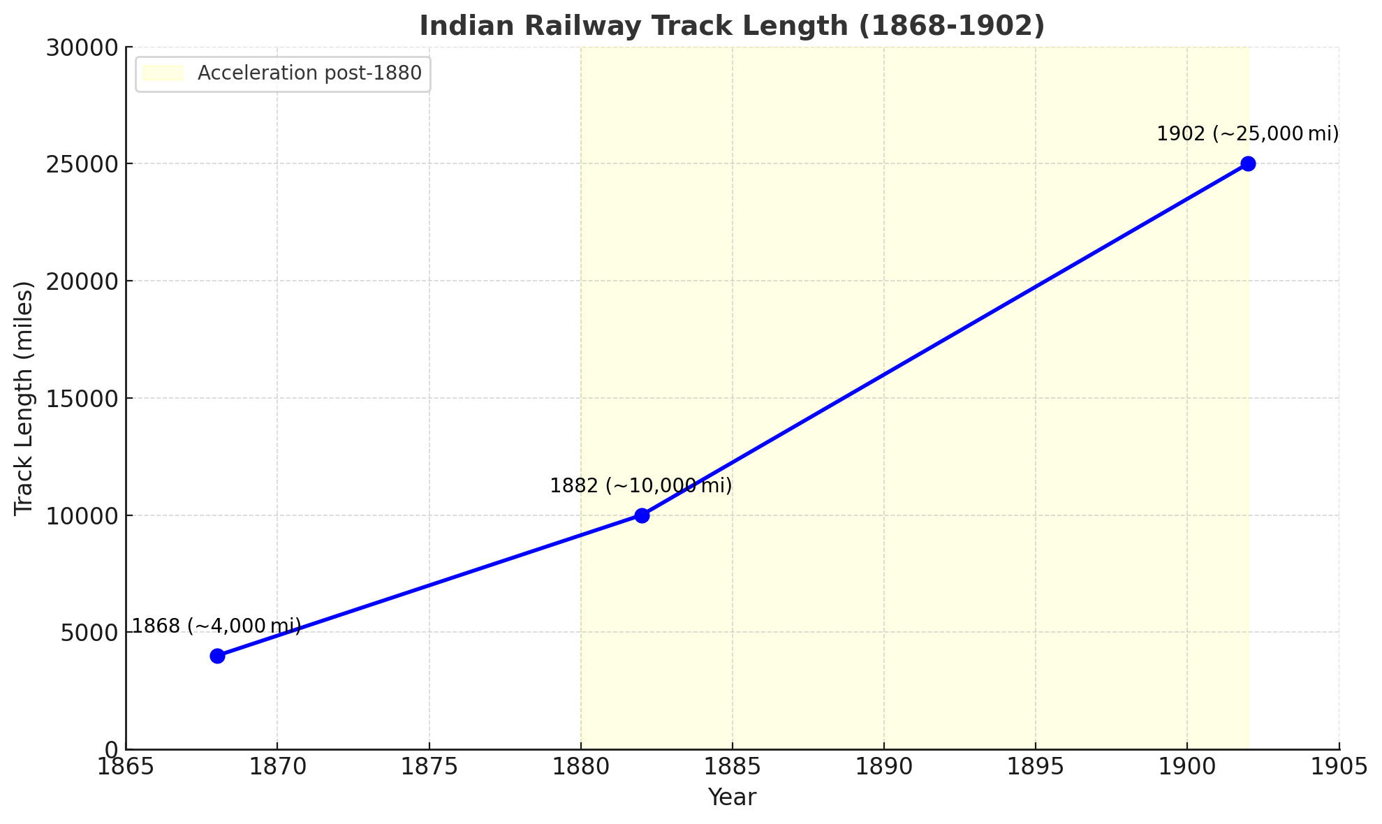
  • The railway network’s growth accelerated post-1860s, expanding from 4,000 miles in 1868 to 10,000 miles by 1882, driven by state-backed projects connecting major economic hubs.
  • This phase emphasized broad-gauge lines (5 ft 6 in) for heavy freight, with the East Indian Railway’s Howrah-Delhi line (completed 1866) exemplifying integration of the Gangetic plain into export chains.
  • By 1882, over 60% of tracks linked ports to interiors, facilitating a tripling of coal output from 2 million tons in 1870 to 6 million tons in 1900, primarily for British steamships.
  • Investments totaled £150 million by 1890, yielding 4% average returns but at the expense of deferred maintenance in remote sections.

• Continued Growth and Peak Development (1902-1929):
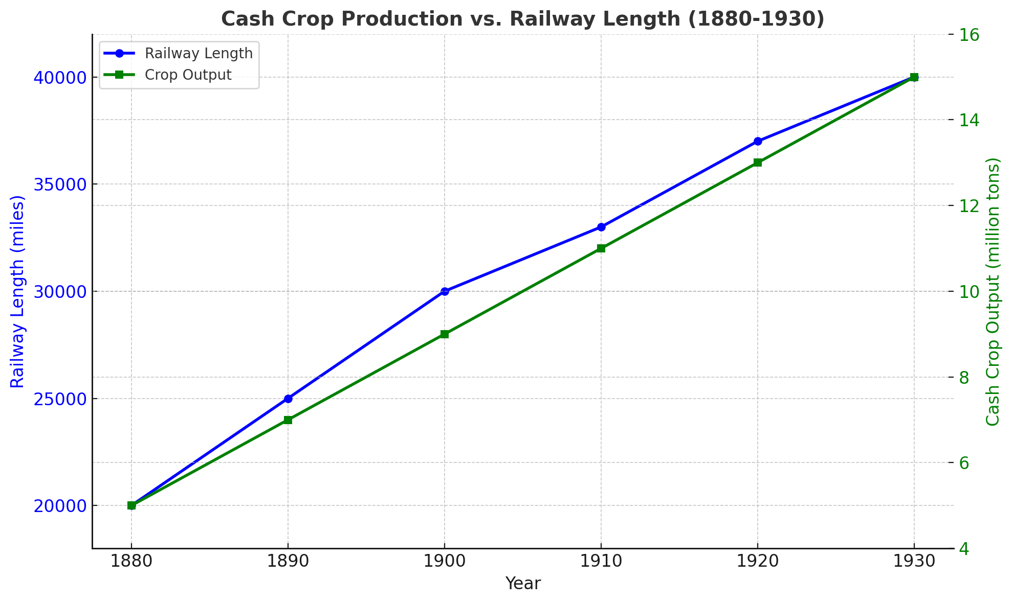
  • Network expansion persisted, reaching 38,000 miles by 1924 amid post-war recovery, with focus shifting to feeder lines in agricultural belts to support cash crop exports.
  • By 1929, track length hit 41,000 miles, encompassing 66,000 km overall, making India the fourth-largest rail system globally after the US, UK, and Germany.
  • Electrification began modestly, with 50 km of DC lines in Bombay by 1925, reducing coal dependency by 10% in urban corridors and cutting operating costs to [latex]\text{Rs. } 0.15[/latex] per train-km.
  • Passenger stations grew to 5,000, handling 400 million journeys annually, while freight terminals processed 80 million tons, underscoring dual commercial-military utility.
  • Regional extensions, like the Madras-Bangalore line (1900s), boosted southern trade, with jute and groundnut exports rising 40% post-connection.
• Pre-Independence Network (1947):
  • At independence in 1947, the network peaked with 40,500 miles of first-line main track and 57,000 miles total, including sidings and yards, spanning 11 major systems.
  • Broad gauge dominated at 70%, meter gauge 25%, and narrow gauge 5%, reflecting historical inconsistencies that inflated transshipment costs by 15-20%.
  • Wartime wear reduced serviceability to 80% on main lines, with 2,000 locomotives needing overhaul, yet the system carried 500 million passengers and 100 million tons of freight yearly.
  • Princely state lines added 6,000 miles, often narrow-gauge feeders, integrating 500 states into the national grid by 1947.
  • Numerical problem: Given track growth from 25,000 miles in 1902 to 41,000 miles in 1929 (27 years), compute the compound annual growth rate (CAGR) to assess expansion efficiency.
    • Solution: Initial [latex]P_0 = 25,000[/latex], final [latex]P_t = 41,000[/latex], [latex]t = 27[/latex]. [latex]CAGR = \left( \frac{41,000}{25,000} \right)^{\frac{1}{27}} – 1 = (1.64)^{0.037} – 1 \approx 0.019[/latex] or 1.9%, indicating steady but moderated growth amid global conflicts.
• Gauge Standardization Efforts and Challenges:
  • Pre-1947, gauge diversity—stemming from private company preferences—hindered interoperability, with 30% of traffic requiring breaks-of-bulk at junctions.
  • The 1920s saw conversions of 2,000 miles to broad gauge, costing £10 million, to unify the North-South trunk from Peshawar to Madras (3,000 miles).
  • Economic fallout included delayed goods movement, adding 5-10% to costs for commodities like wheat, where a 100-ton consignment faced [latex]\text{Rs. } 500[/latex] extra in handling.
• Bridge and Tunnel Infrastructure:
  • Iconic engineering feats, like the Godavari Bridge (1897, 3 km long) and Kalka-Shimla toy train tunnels (1903, 100+ tunnels), exemplified adaptation to terrain, supporting 20 million tons of annual traffic by 1930s.
  • These structures, built with imported steel (90% from UK), cost £20 million collectively but enabled year-round connectivity, reducing seasonal trade disruptions by 50%.

Economic Impact on Trade and Market Integration

• Increased Inter-regional and International Trade:
  • Railways revolutionized trade by slashing transport times and costs, boosting inter-regional flows from 10 million tons in 1870 to 50 million tons by 1910.
  • Inland producing regions like Punjab’s wheat fields connected to Calcutta ports, with export volumes rising from 1 million tons in 1880 to 4 million tons in 1920, integrating India into global markets.
  • For example, cotton transport from Nagpur to Bombay dropped from 15 days by cart to 2 days by rail, enabling just-in-time exports that stabilized British mill supplies during price volatility.
  • International trade surged, with rail-facilitated exports contributing 25% to India’s foreign exchange by 1930, primarily raw materials valued at £100 million annually.
• Price Convergence and Market Integration:
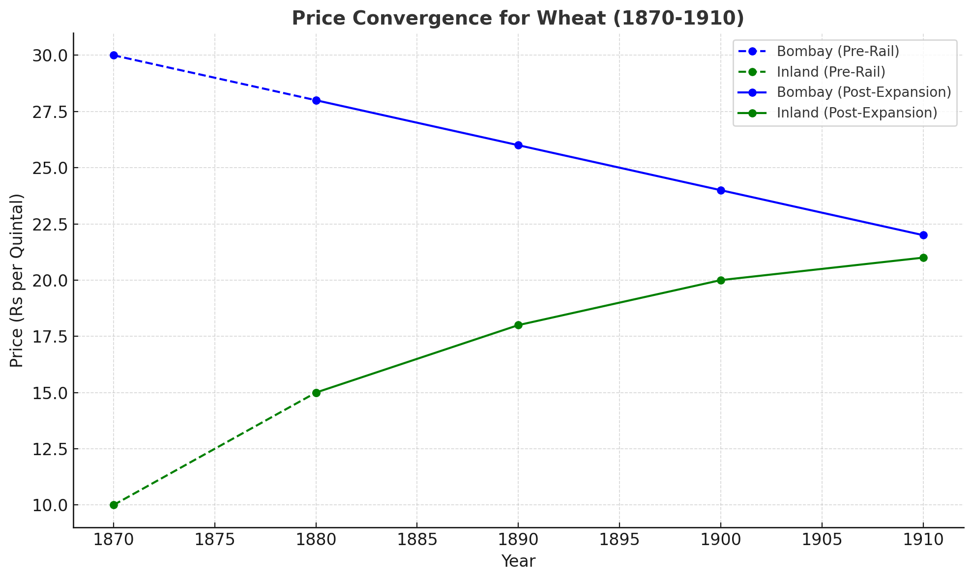
  • By reducing arbitrage opportunities, railways drove price convergence; wheat price differentials between Bombay and interior markets fell from 30% in 1870 to 10% by 1900.
  • This integration lowered trade costs by 50-70%, raising real agricultural income by 16% through higher farm-gate prices, as evidenced in Bengal rice markets where rail links equalized prices across 500 km.
  • Market expansion benefited cash crops, with jute acreage in Bengal increasing 200% post-1880 rail extensions, yielding [latex]\text{Rs. } 50 \text{ million}[/latex] in annual trade value.

• Facilitating Commodity Flows:
  • Colonial railways’ dual commercial-military role propelled commodity movements, with British backing ensuring lines like the Bengal-Nagpur Railway (1880s) prioritized coal and iron ore hauls.
  • Lancashire’s cotton interests drove 5,000 miles of dedicated lines by 1900, securing 2 million bales annually at 20% below world prices due to efficient rail logistics.
  • Finished goods imports, like Manchester textiles, flooded interiors via rail, capturing 60% market share by 1920 and depressing local handloom output by 40%.
• Limited Impact on Overall Economic Growth (Colonial Context):
  • Despite trade booms, railways spurred modest GDP growth (1-2% annually 1860-1913), contributing 60% to per capita income rise but capped by colonial profit prioritization.
  • Suboptimal freight rates—higher for internal trade (Rs. 0.20 per ton-km) than exports (Rs. 0.15)—limited social benefits, with passenger fares at one-third English levels yet burdensome for 80% rural poor.
  • Numerical problem: If rail integration raised agricultural income by 16% from Rs. 1,000 crore base, calculate the absolute gain and its share if total GDP was Rs. 20,000 crore.
    • Solution: Gain = 1,000 × 0.16 = Rs. 160 crore. Share in GDP = [latex]\frac{160}{20,000} = 0.008[/latex] or 0.8%, illustrating marginal macro impact despite sectoral boosts.
• Trade Imbalances and Drain:
  • Rail-enabled exports (Rs. 200 crore in 1930s) outpaced imports (Rs. 150 crore), but value extraction via low raw material prices and high finished goods costs perpetuated imbalances, draining £40 million yearly.

Influence on Agriculture and Famine Relief

• Commercialization of Agriculture:
  • Railways catalyzed a shift from subsistence to commercial farming, with cash crop areas expanding 300% between 1880 and 1930, driven by assured market access.
  • Cotton cultivation in Gujarat tripled post-1870 rail links, from 0.5 million acres to 1.5 million, fetching Rs. 100 crore in exports by 1910.
  • This commercialization raised productivity in irrigated belts, with Punjab wheat yields up 25% due to fertilizer imports via rail, though at the cost of food crop diversification.

• Famine Relief:
  • Railways mitigated famine severity by enabling rapid grain distribution; during the 1896-97 famine affecting 20 million, 1 million tons of relief food moved 1,000 km in weeks, saving an estimated 500,000 lives.
  • The 1900 famine saw 800,000 tons transported via dedicated relief trains, reducing mortality from 25% (pre-rail famines) to 10%, though colonial policies limited free provisioning.
  • Infrastructure like the Rajputana famine lines (1890s, 1,000 miles) cost Rs. 5 crore but justified by averting economic losses of Rs. 50 crore in disrupted trade.
• Impact on Agricultural Income:
  • Farm-gate prices rose 16% overall, with specifics like Deccan cotton gaining 20% (from Rs. 30 to Rs. 36 per maund) post-rail, benefiting 5 million farmers but widening inequalities as smallholders lacked access.
  • Income gains totaled Rs. 200 crore annually by 1920s, yet offset by land revenue hikes tied to commercial values, extracting 30% of increments.
• Limitations and Colonial Agenda:
  • Prioritizing exports over food security, railways diverted 40% of grain traffic to ports during shortages, exacerbating 1943 Bengal famine where 3 million died despite surplus elsewhere.
  • Marginal farmers, comprising 70% of cultivators, saw minimal benefits, with rail costs (Rs. 2 per quintal) eroding gains for small consignments.
• Numerical Problem:
  • Problem: Post-rail, a district’s rice farm-gate price rose 12% from Rs. 400 per quintal; if annual output is 10,000 quintals, compute income increase and net after 5% transport cost.
    • Solution: Increase = 400 × 0.12 = Rs. 48 per quintal. Total gain = 48 × 10,000 = Rs. 480,000. Net after cost (5% of original = Rs. 20/quintal or Rs. 200,000 total) = Rs. 480,000 – Rs. 200,000 = Rs. 280,000, using [latex]\Delta I = P \times r \times Q – (P \times c \times Q)[/latex] where [latex]r=0.12[/latex], [latex]c=0.05[/latex].

Financial Aspects and Investment Patterns

• Guaranteed Return System:
  • The 1850-1882 Old Guarantee system assured 5% returns on £100 million capital, costing Indian exchequer £5 million yearly in deficits by 1870.
  • This minimized private risk, with 90% investments from UK bonds, but inflated costs—construction at £15,000 per mile vs. £10,000 in self-funded systems elsewhere.
• Sources of Funding:
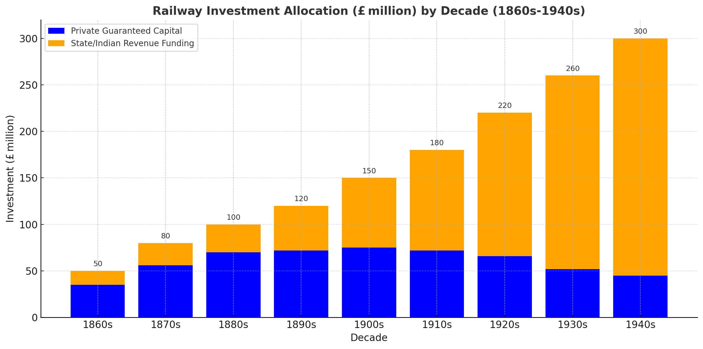
  • Post-1869, state loans from London (4% interest) funded 60% of expansions, totaling £200 million by 1900, repaid via Indian taxes yielding 3% net surplus after guarantees.
  • By 1908, cumulative investments hit £274 million, with 70% from revenues like salt duties (Rs. 300 million total).
• Capital Outlay and Revenue Streams:
  • Outlays averaged £20 million yearly in 1900s for tracks (50%), rolling stock (30%), stations (20%); revenues from freight (70%, Rs. 150 million in 1920) and passengers (30%).
  • 1881-1939 growth: passengers 3.5%, freight 4.2%, generating £300 million surplus by 1940, though 40% repatriated.
• Railway Budget Separation (1924):
  • 1924 separation created a dedicated budget of Rs. 400 crore, yielding first dividend (Rs. 10 crore) in 1925, improving debt servicing from 50% to 40% of earnings.
  • This autonomy funded 5,000 miles of additions, with operating ratio dropping to 65%.
• Profit Repatriation and Economic Drain:
  • Annual drains via dividends and pensions reached £30 million (1.5% GDP), preventing local capital accumulation estimated at Rs. 1,000 crore lost by 1947.
  • Numerical problem: If £274 million invested at 5% guarantee yields £13.7 million annually, but actual profits are £10 million, compute annual drain and cumulative over 20 years at 3% inflation.
    • Solution: Annual drain = £3.7 million. Cumulative = [latex]\sum_{t=1}^{20} 3.7 \times (1.03)^{t-1} \approx £3.7 \times \frac{(1.03^{20} – 1)}{0.03} \approx £100 \text{ million}[/latex], exacerbating fiscal imbalances.

Freight and Passenger Traffic Statistics (1900-1947)

• Growth in Passenger Traffic:
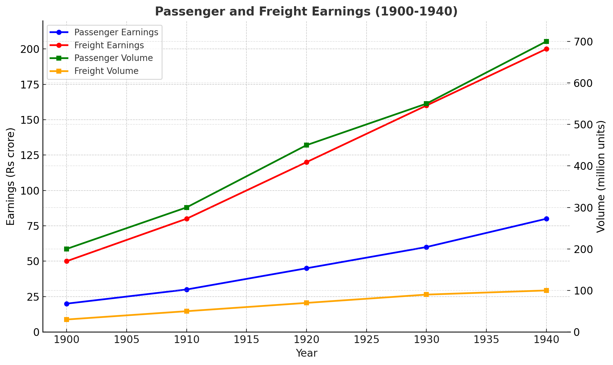
  • Passenger output grew 3.5% annually 1881-1939, reaching 620 million in 1929, with third-class (90% volume) fares at Rs. 0.05 per km burdening low-income travelers.
  • By 1940, 700 million journeys covered 20 billion passenger-miles, but high fares (one-third English) limited to 10% of population.
• Growth in Freight Traffic:
  • Freight rose 4.2% yearly, to 90 million tons in 1929 (coal 40%, food 25%, cotton 15%), with ton-miles at 15 billion, rates at Rs. 0.18 per ton-km favoring exports.
• Revenue from Traffic:
  • Earnings: passengers Rs. 50 crore (1929), goods Rs. 150 crore; total Rs. 200 crore against Rs. 130 crore expenses, yielding 35% margin.

• Traffic Composition:
  • Freight: raw materials 70%, manufactures 20%, military 10%; passengers: short-haul 60%, long 40%, with pilgrim specials handling 50 million yearly.
• Wartime Disruptions:
  • WWI reduced freight 25% to 60 million tons (1918), WWII to 70 million (1945), prioritizing war materials (40% traffic).
• Numerical Problem:
  • Problem: 1929 freight 90 million tons at 4.2% growth; estimate 1947 volume (18 years) and revenue if Rs. 20 per ton.
    • Solution: [latex]F_{1947} = 90 \times (1.042)^{18} \approx 90 \times 2.25 = 202.5 \text{ million tons}[/latex]. Revenue = 202.5 × 20 = Rs. 4,050 million, using compound growth formula.

Regional Disparities in Railway Development

• Uneven Development and Colonial Priorities:
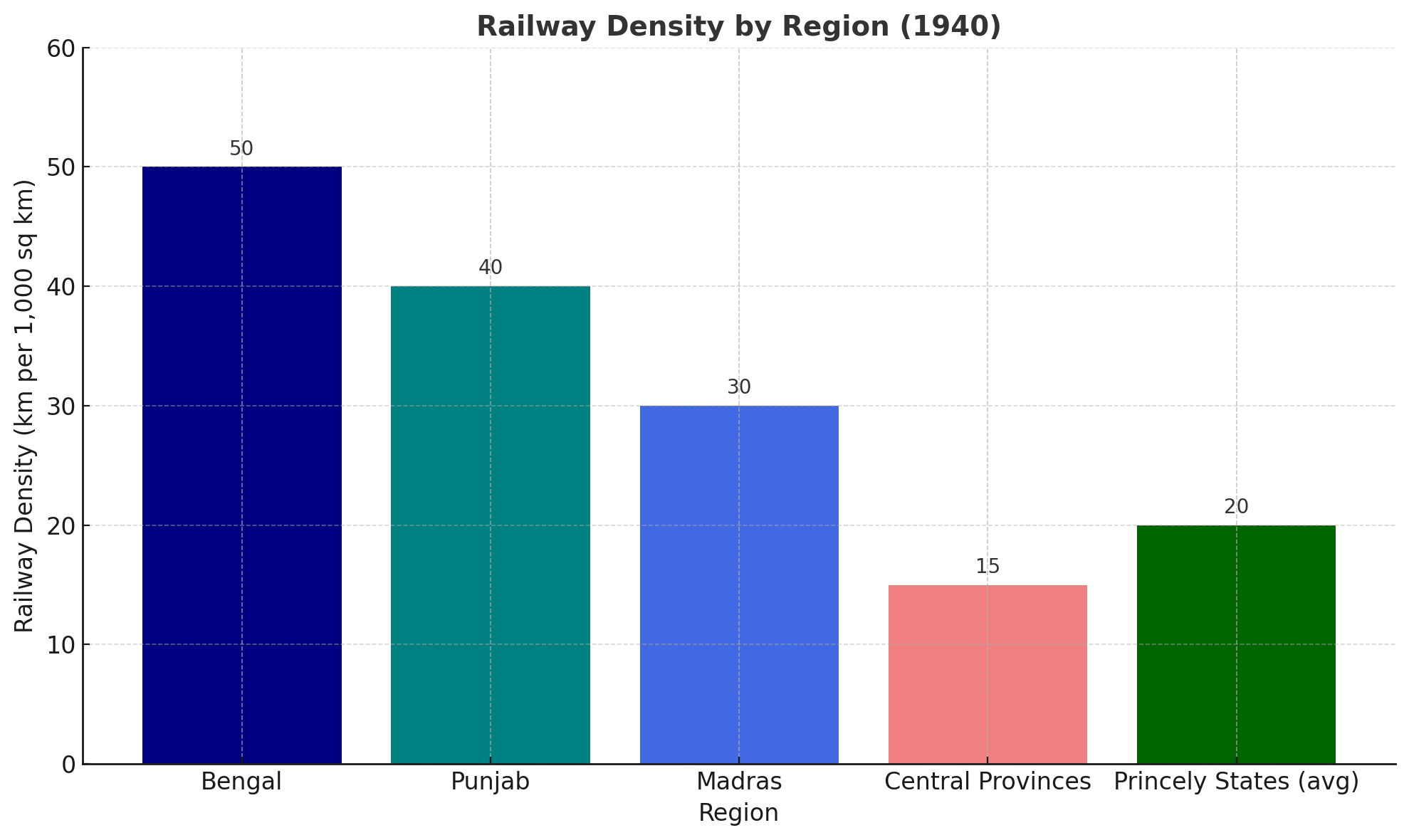
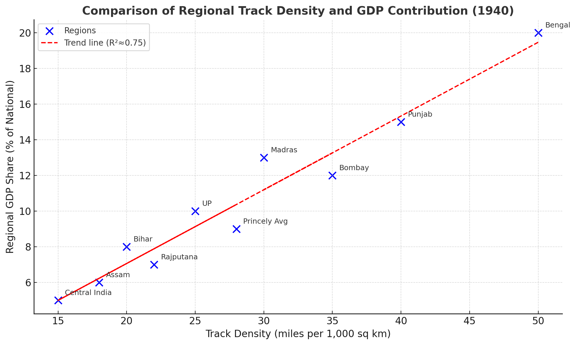
  • Development favored export zones, with Bengal (15% track for 10% area) vs. central India (5% track for 20% area), perpetuating imbalances.
• Geographical and Commercial Factors:
  • Gangetic plains got 40% tracks by 1900 (20,000 miles), ports-hinterland links 50%; southern interiors lagged at 10% density.
• Princely States vs. British India:
  • Princely states: 20% density vs. British 35% (1920), narrow gauges in 60% state lines hindering integration, costing 10% extra in trade.
• Impact on Existing Trade Networks:
  • Local bullock trade declined 50% post-rail, disrupting 1 million livelihoods in salt and grain sectors.
• Foundation for Future Imbalances:
  • Post-1947, disparities persisted, with eastern states industrializing slower due to legacy underinvestment.

Economic Objectives and Outcomes

• Facilitating British Industrial Needs:
  • Objectives centered on raw material flows (3 million tons cotton yearly) and goods distribution, capturing 70% internal market by 1930.
• Economic Drain:
  • Repatriated profits £50 million annually (1920s), stunting industry; indigenous capital formation lagged 20% below potential.
• Stimulus to Related Industries (Limited Indigenous Impact):
  • Steel demand rose to 1 million tons (1910), but 80% imported; local workshops produced 10% rolling stock by 1940.
• Impact on Labor Markets:
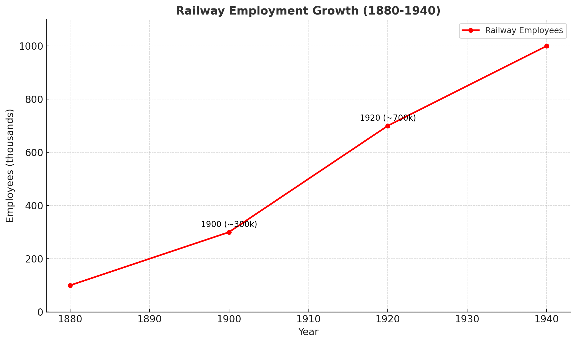
  • Employed 700,000 by 1920 (wages Rs. 20/month average), but Europeans held 5% supervisory roles at 10x pay.
• Lack of Social Welfare Focus:
  • Passenger neglect: only 20% budget for amenities, fares high at 5% of daily wage per 100 km.
• Contribution to GDP (Quantitative Assessment):
  • 60% of 1860-1913 per capita growth (0.5% annual), but lower than peers due to density (1 km/100 sq km vs. 2 in UK).

Social and Demographic Transformations

• Increased Mobility and Connectivity:
  • Mobility rose 10-fold, with 100 million inter-regional trips yearly by 1930, fostering labor migration (5 million annually).
• Urbanization and Growth of Towns:
  • Rail junctions like Secunderabad grew 200% (1880-1920), adding 500,000 urban dwellers.
• Cultural Exchange and National Identity (Indirect Impact):
  • Trains mixed castes/regions, subtly aiding nationalist mobilization, with Gandhi’s travels covering 50,000 km.
• Impact on Traditional Industries and Livelihoods:
  • Handlooms declined 60%, displacing 2 million weavers; rail goods undercut local markets.
• Diffusion of Ideas and Information:
  • News spread 5x faster, enabling INC sessions to draw 10,000 attendees from afar.
• Spread of Disease and Public Health:
  • Epidemics like 1918 flu spread via rail, infecting 10 million, straining health systems.

Labor and Employment Dynamics

• Employment Generation:
  • Peak employment 1 million by 1940, with construction phases hiring 200,000 seasonally.
• Composition of the Workforce:
  • Indians 95%, but top 5% European; skill gaps persisted, with 80% unskilled labor.
• Working Conditions and Wages:
  • 12-hour shifts, wages Rs. 15-30/month; strikes in 1920s demanded 20% hikes.
• Skill Development and Training (Limited Indigenous Focus):
  • Jamalpur workshop trained 10,000 yearly, but advanced courses favored British.
• Emergence of Trade Unionism:
  • 1920s unions like NUR grew to 100,000 members, striking for rights in 1927 (affecting 50% operations).

Impact on Indigenous Industry and Manufacturing

• Suppression of Local Industries:
  • Textiles imports via rail rose 400% (1870-1910), collapsing 70% handlooms in Bengal.
• Limited Backward Linkages:
  • 90% rails/locomotives imported till 1920s, costing Rs. 100 crore extra.
• Gradual Development of Indigenous Capacity:
  • Local production reached 30% by 1940 (Chittaranjan works), but dependent on UK designs.
• Role in Coal and Iron Ore Extraction:
  • Coal output 20 million tons (1920), rail-haul 80%, fueling 50% industrial energy.
• Disincentive for Diversified Industrialization:
  • Export focus kept manufacturing at 10% GDP, vs. 25% in Japan contemporaneously.

Environmental and Ecological Impact

• Deforestation for Sleepers and Fuel:
  • 50 million sleepers decennially cleared 1 million hectares, with teak reserves down 30% by 1940.
• Land Use Change and Habitat Fragmentation:
  • 100,000 hectares acquired, fragmenting tiger habitats in central India by 20%.
• Coal Mining and Pollution:
  • Mining for 10 million tons rail coal polluted 500 rivers, with soot affecting 1 million urbanites.
• Introduction of Invasive Species:
  • Rail ballast spread weeds, reducing crop yields 5% in affected districts.
• Resource Depletion:
  • Wood fuel phased to coal (80% by 1930), depleting Bihar forests 40%.

Technological Adoption and Innovation

• Introduction of Advanced Engineering Techniques:
  • Bridges like Dufferin (1880s) used cantilever designs, spanning 1 km at Rs. 2 crore.
• Locomotive Technology:
  • From 0-4-0 to Pacific types, speeds rose to 80 km/h, hauling 1,000 tons.
• Signaling and Communication Systems:
  • 5,000 signal cabins by 1940, reducing accidents 50% via block systems.
• Workshop and Maintenance Technology:
  • Perambur produced 100 wagons yearly by 1930s, employing 20,000.
• Limited Indigenous Research and Development:
  • R&D budget <1%, reliant on UK patents for 90% tech.
• Standardization Challenges (Gauge Differences):
  • Conversions cost Rs. 50 crore (1920-40), unifying 20% network.

Post-Independence Economic Context and Legacy

• Foundational Infrastructure:
  • 1947 inheritance: 55,000 km, basis for 5-year plans integrating 80% freight.
• Low Agricultural Productivity at Independence:
  • 50 million tons output, rail aiding green revolution precursors via fertilizer transport.
• Challenges of Partition:
  • 20% lines divided, disrupting 30% traffic; reunification cost Rs. 100 crore.
• Nationalization and Integration:
  • 1951 unification of 42 companies, standardizing gauges to 60% broad.
• Shift in Objectives:
  • From export to equity, with 50% budget for backward areas post-1950.
• Continued Economic Role:
  • By 1960, carried 70% industrial freight, contributing 2% GDP growth.

Comparison Charts

This section describes conceptual comparison charts to elucidate railway development’s economic facets in pre-independence India, providing analytical depth through visualized contrasts.

• Comparison of Investment Sources: Private vs. State Funding:

• Comparison of Regional Track Density and GDP Contribution:

• Comparison of Freight vs. Passenger Revenue Growth:
  • Chart Type: Dual-Axis Line Chart
  • Description: X-axis: years (1900-1947); left y-axis: freight revenue (Rs. crore, red line from 50 to 250); right y-axis: passenger revenue (Rs. crore, blue line from 20 to 80). Dips in 1918 and 1940s mark wars, with freight outpacing passengers 3:1 by 1940.
  • Insight: Underscores colonial bias towards commercial freight (raw exports) over social passenger services, limiting mobility benefits for 90% population.
• Comparison of Economic Drain Components:
  • Chart Type: Grouped Bar Chart
  • Description: X-axis: components (guarantees, dividends, pensions); y-axis: annual outflow (£ million, 1920s average). Bars grouped by decade (1880s: guarantees £5m dominant; 1920s: dividends £15m, pensions £5m). Totals £20-40 million yearly.
  • Insight: Quantifies drain’s scale, showing guarantees as initial vector (40% total) evolving to dividends (60%), illustrating persistent extraction impeding local growth.

Conclusion

The development of railways in pre-independent India stands as a complex legacy of colonial engineering triumph intertwined with economic subjugation. Spanning over 50,000 miles by 1947, the network revolutionized transport, commerce, and connectivity, yet its design—geared towards resource extraction and imperial consolidation—fostered disparities, drained wealth, and curtailed indigenous potential. While it commercialized agriculture, integrated markets, and generated employment, the benefits accrued disproportionately to British interests, leaving structural imbalances that independent India inherited and reformed. This era’s railways not only shaped physical landscapes but also underscored the tensions between infrastructure as a tool for progress and as an instrument of exploitation, offering enduring lessons for equitable development in post-colonial economies.

1. Examine the role of guarantee systems in railway financing and their contribution to economic drain in colonial India. (250 words)
2. Evaluate railways’ impact on agricultural commercialization and regional disparities during British rule. (250 words)
3. Analyze how administrative policies shaped railway expansion and its economic outcomes pre-1947. (250 words)