
5.1.1 Harrod’s Growth Model | Theories of Economic Growth
Introduction: Harrod’s Growth Model is a Keynesian theory of economic growth linking an economy’s expansion to savings and investment. Developed by Roy F. Harrod in 1939, it was among the first Keynesian models to analyze long-run growth. Harrod’s framework introduced the concept of a warranted growth rate – the equilibrium GDP growth rate when all saving is absorbed by investment – alongside a natural growth rate governed by labor force growth (and technological progress). It highlighted the possibility of an unstable equilibrium growth path, often referred to as the “knife-edge” problem, where even small deviations can lead to boom or bust.
1. Historical Background and Context
- Origins in the Keynesian Era: Harrod’s model emerged from the intellectual climate of the late 1930s, as economists sought to extend Keynesian analysis beyond short-term fluctuations to long-term growth. Harrod published his seminal “Essay in Dynamic Theory” in 1939, attempting to formulate a dynamic growth analog to Keynes’s static equilibrium.
- Earlier, John Maynard Keynes had focused on short-run output determination (in The General Theory, 1936), leaving open the question of what determines an economy’s growth rate over years and decades. Harrod, a close colleague of Keynes, took up this challenge.
- Around the same time (1946), economist Evsey Domar independently developed a similar growth model. Because of their complementary insights, the combined framework is often called the Harrod-Domar model. Harrod’s exposition placed more emphasis on growth rate concepts and instability, while Domar focused on the dual role of investment (as a creator of capacity and generator of demand).
- Earlier growth thinking: Before Harrod, classical economists like Adam Smith and David Ricardo had discussed growth in terms of capital accumulation, labor, and land, but largely from a supply-side perspective (e.g., diminishing returns in agriculture leading to a stationary state). There was no formal macroeconomic model for sustained growth rates. The interwar period saw economist Joseph Schumpeter emphasize innovation and business cycles rather than a steady growth path. Harrod’s contribution was novel in that he attempted to write down explicit growth equations in the spirit of Keynesian economics, which put aggregate demand at center stage.
- Harrod’s ideas were first presented in “An Essay in Dynamic Theory” (1939). Evsey Domar’s parallel analysis came in a 1946 paper “Capital Expansion, Rate of Growth, and Employment.” Because their equations and implications were so similar, the model became known jointly as Harrod-Domar. This Keynesian approach to growth contrasted with later neoclassical models (Solow, 1956) which took a different route, as we will see, but it set the agenda by highlighting that ensuring sufficient investment demand over time is critical for an economy’s health.
- Early Reception and Significance: Harrod’s theory was groundbreaking as one of the first formal models of economic growth. It shifted attention to long-run equilibrium growth paths at a time when classical economists had left growth largely to exogenous factors.
- The model underscored the importance of savings and investment as primary drivers of growth. Unlike earlier classical views (which emphasized technology or capital accumulation qualitatively), Harrod provided a quantitative link between the savings rate and the growth rate needed to maintain equilibrium.
- Harrod’s work, together with Domar’s, laid the foundation for post-war development economics. Newly independent countries (including India) found the model attractive for guiding economic planning, as it suggested that boosting savings and investment could directly accelerate growth.
- By the 1950s, however, questions arose about the model’s implications, especially its apparent instability. This spurred further research – most notably the Solow-Swan neoclassical growth model (developed in the mid-1950s) – as economists sought a more stable growth mechanism. Nonetheless, Harrod’s concepts of warranted and natural growth remained influential.
- Harrod’s work was also colored by recent history: the Great Depression of the 1930s had demonstrated how economies could suffer prolonged underemployment equilibrium, and World War II showed that massive government investment could mobilize idle resources. Thus, a pressing question was how to ensure full employment growth in peacetime. Harrod’s model directly grappled with this, essentially extending Keynes’s analysis (which explained short-run underemployment) into a long-run growth scenario. The specter of insufficient investment leading to stagnation, versus excessive investment causing inflation, was not just theoretical – it was informed by the economic turbulence of the first half of the 20th century.
- Context in Economic Thought: Harrod’s Growth Model came on the heels of the Great Depression and World War II, when achieving full employment and rebuilding economies were paramount.
- The theory offered a way to think about the long-term trajectory of an economy’s output, not just short-run cycles. This was a significant contribution, as it started the formal analysis of growth dynamics which later blossomed into growth theory as a distinct field.
- It also dovetailed with early development planning: countries with capital scarcity interpreted the model as justification for aggressive investment drives, foreign aid (to fill the “savings gap”), and government planning to reach a desired growth path.
- In India, for example, planners in the 1950s adopted frameworks reminiscent of Harrod-Domar – using the concept of a fixed capital-output ratio and required investment rate – to set targets for GDP growth in the Five-Year Plans.
2. Fundamental Assumptions and Setup
- Single good economy (one-sector model): Harrod’s model considers a simplified economy producing a single composite output (like aggregate GDP) which can be consumed or invested. It assumes a closed economy with no government intervention, so there are no foreign trade effects or fiscal policies – all output not consumed is saved and invested domestically.
- This implies that total saving equals total investment (S = I) in equilibrium, as there are no external leakages or injections. The model abstracts from government spending or taxation, focusing purely on private sector behavior.
- The single-sector focus means the entire economy can be summarized by aggregate production and expenditure, without modeling different industries separately. This is a “macro” model treating the economy in aggregate terms.
- Constant saving rate: A core assumption is that a fixed proportion of income is saved. Let s denote the marginal (and average) propensity to save, which is exogenously given and remains constant over time (e.g., if s = 0.25, households save 25% of any income level).
- As a result, Savings (S) at any level of output Y is given by S = s·Y. For example, if national income is ₹100 lakh crore and s = 0.3, then S = 0.3 × 100 = ₹30 lakh crore saved.
- This treats saving behavior as stable and independent of short-run fluctuations. It ignores potential changes in saving rates as income grows or as interest rates change. The simplicity allows linking saving directly to investment and growth.
- Capital-driven production (labor assumed abundant): The model assumes output is determined solely by the capital stock. Labor and other factors are either considered in unlimited supply or used in fixed proportion to capital. Formally, output (Y) is assumed to be a linear function of capital (K):
- One common formulation is a fixed capital-output ratio v, meaning K = v·Y. Equivalently, for every unit of output, v units of capital are required. The productivity of capital is thus constant. (If v = 4, then ₹4 of capital produces ₹1 of output. The reciprocal 1/v = 0.25 is the marginal product of capital.)
- Because of this fixed-proportions production function, the marginal and average product of capital are equal and constant. If one machine (unit of capital) always adds the same amount to output, there are no diminishing returns to capital in this model. For instance, whether the economy has ₹100 crore of capital or ₹1000 crore, each ₹1 crore of capital might consistently produce say ₹0.2 crore of output if the capital-output ratio is constant at 5.
- This assumption effectively ignores labor as a limiting factor in the short run – it presumes that there is sufficient labor to work with the available capital at the given capital-output ratio. In other words, labor will not constrain output unless specifically introduced via the “natural rate of growth” (which deals with labor force growth externally).
- Fixed technology and constant returns: Technological progress is either absent or embedded in the constant relationship between capital and output. The production function exhibits constant returns to scale – doubling capital (and implicitly labor in the same proportion) would double output.
- Harrod’s model does not explicitly incorporate technological change as an internal element. Any improvements in technology would effectively alter the capital-output ratio, but in the basic model v is treated as given and unchanging in the analysis.
- Because technology is not explicitly modeled, the only way to grow output is by accumulating more capital (and employing more labor if available). This is a distinguishing feature from later models (like Solow’s), where technological progress plays a central role.
- Full utilization of capital (and initial full employment): It is assumed that in equilibrium the economy utilizes its capital stock fully (no idle factories or machines when operating on the warranted growth path). Often the model also assumes the economy begins at full employment of labor and capital, so the analysis focuses on maintaining that state.
- Full utilization means the capital-output ratio v reflects normal use of capacity. If K = v·Y, all installed capital is producing output as per the ratio. There are no general gluts or shortages at the starting point.
- By assuming an initial situation of full employment of resources, Harrod can examine what conditions are needed to keep the economy growing without slipping into unemployment or overcapacity. It sets a benchmark for “steady growth” from a position of balance.
- No price flexibility to clear markets: In line with Keynesian tradition, prices (especially wages and the interest rate) are not assumed to adjust to equilibrate saving and investment automatically. Planned saving may not equal planned investment unless the growth rate happens to be at the warranted level.
- Wages are often considered rigid in the short run, so any excess labor supply won’t immediately drive wages down to restore full employment (this underpins the significance of the natural growth rate constraint).
- The interest rate’s role in equalizing saving and investment is downplayed; investment is driven by expectations of growth rather than flexible interest adjustments. This is why the model can result in disequilibrium growth if not properly managed.
- Investment creates capacity instantly: Implicitly, new investment spending adds to the capital stock without significant gestation lags in this model. When firms invest, that capital becomes available to produce output in the next period.
- In reality, building new factories or infrastructure takes time, but Harrod’s model abstracts from such lags to focus on overall growth trends. This simplification means that an increase in investment immediately contributes to higher productive capacity (K) and thus potential output.
- It also implies that entrepreneurs plan their investment based on expected growth in demand; if those expectations are met, capital stock and output grow in tandem. If expectations are off, however, it leads to the instability issues discussed later.
- Time horizon and dynamics: Harrod’s analysis is dynamic, looking at growth year after year (or period after period). However, it often uses a discrete or continuous time approach with relatively short time intervals to examine whether the economy can keep on a steady trajectory.
- The model’s equations can be written in discrete annual terms or in calculus form (with growth rates as derivatives). In either case, it’s about how variables change over time rather than a static snapshot.
- The key dynamic variables are output (Y) and capital (K). Their growth over time will be determined by saving/investment behavior and the fixed ratio linking K and Y.
- Note on depreciation: Many expositions of the Harrod-Domar model assume, for simplicity, that capital does not depreciate (or that depreciation is already netted out in the capital-output ratio). If depreciation (at rate δ) is considered, the net growth formula would be slightly modified (investment must not only create new capital but also replace depreciated capital).
- Including depreciation means the net addition to capital is I – δ·K. The equilibrium condition would then require that net investment equals the amount needed to expand output. In formula form, the warranted growth rate would be g_w = (s/v) – δ, because part of saving goes to make up for worn-out capital.
- However, for clarity in derivations, the model is often discussed in terms of net output and net investment (after depreciation) or assumes δ is small enough to be omitted initially. We will proceed primarily with the simpler case where all investment effectively adds to capacity.
3. Saving–Investment Dynamics and Output Growth
- Savings equals investment (accounting identity): In this model, with no government or foreign trade, all income not consumed is saved, and all saving flows into investment. Thus, ex post saving (S) always equals ex post investment (I). The equality can be written as:
- [latex]S = I[/latex] (by definition in a closed economy with no government)
- However, this identity doesn’t guarantee that planned (ex ante) saving equals planned investment at all times – that equality only holds when the economy grows at a particular rate (the warranted rate, discussed soon). For now, S = I simply reflects that whatever is invested must come from someone’s saving.
- Saving function: As per the assumptions, saving is a constant fraction of income:
- [latex]S = s , Y[/latex], where 0 < s < 1 is the saving rate. (Equation 1)
- For example, if s = 0.20 and national income Y = ₹200 lakh crore, then S = 0.20 × 200 = ₹40 lakh crore is saved and invested.
- This linear saving function implies that higher income leads to proportionally higher saving, providing more funds for investment to fuel growth.
- Investment and capital accumulation: Investment (I) is defined as the addition to the capital stock. If ΔK denotes the increase in capital stock in a year (net of depreciation), then:
- [latex]I = \Delta K[/latex]. (Equation 2)
- For instance, if firms invest ₹50,000 crore in new factories and machines this year, the capital stock K increases by that amount (assuming depreciation is accounted for or negligible in this context).
- Investment not only generates demand (as per Keynesian short-run effect) but also expands the economy’s capacity by increasing K, which is crucial for growth in Harrod’s model.
- Fixed capital–output ratio: The link between capital and output is given by a constant capital-output ratio v:
- [latex]K = v , Y[/latex]. This implies a linear production function where one unit of capital yields 1/v units of output. (Equation 3)
- Differentiating or taking a discrete change, the increase in output ΔY requires an investment such that:
- [latex]\Delta K = v , \Delta Y[/latex]. (This comes from assuming the ratio v holds as the economy grows; every extra output needs v times capital.)
- Equation 3 essentially states that to produce ΔY additional output, the economy must accumulate ΔK = vΔY additional capital. For example, if v = 5, an extra ₹1 crore of output requires ₹5 crores of new capital.
- Deriving the Harrodian growth equation: Now combine the above relationships. At equilibrium growth:
- The saving used for investment must equal the new capital required for the output growth. Using S = I and the formulas above:
- [latex]s , Y = \Delta K[/latex] (substituting I and S from Eq.1 and Eq.2)
- [latex]s , Y = v , \Delta Y[/latex] (substituting ΔK from Eq.3)
- Rearranging this, divide both sides by Y: [latex]s = v , \frac{\Delta Y}{Y}[/latex].
- Solve for the growth rate [latex]\frac{\Delta Y}{Y}[/latex]:
- [latex]\frac{\Delta Y}{Y} = \frac{s}{v}[/latex]. (Equation 4)
- This is the fundamental growth relation in the Harrod-Domar model. It says that the actual growth rate of output (ΔY/Y) will equal the saving rate (s) divided by the capital-output ratio (v), as long as the economy is on a steady growth path using all savings productively.
- For example, if a country saves 30% of its GDP (s = 0.3) and each unit of output needs 4 units of capital (v = 4), then the economy could grow at [latex]\frac{0.3}{4} = 0.075[/latex], i.e., 7.5% per year, if it fully utilizes those savings in investment.
- The saving used for investment must equal the new capital required for the output growth. Using S = I and the formulas above:
- Interpretation: The term [latex]\frac{s}{v}[/latex] can be viewed as the potential or warranted growth rate of the economy under those conditions. It reflects the rate of expansion of demand (through investment spending) that matches the rate of expansion of capacity.
- Intuitively, a higher saving rate (s) provides more resources for investment, tending to raise the growth rate. Conversely, a higher capital-output ratio (v) – meaning the economy is “capital intensive” or inefficient, requiring more capital for each unit of output – lowers the growth rate for a given amount of saving.
- This simple formula was very influential. Policymakers could estimate s and v for their economy and get an idea of how fast the economy could grow if all savings are effectively invested. For instance, in India during the 1950s, s was roughly 0.10–0.12 (10–12%) and v was around 3 to 4, yielding a growth potential of only ~3% per year, which matched the slow growth observed. In later decades, as India’s saving rate rose to 0.25–0.30 and efficiency improved (v around 4), the potential growth rose to 6–8%, which indeed was achieved in the 2000s.
- It is important to note that [latex]\frac{\Delta Y}{Y} = \frac{s}{v}[/latex] is an equilibrium result. The actual growth may or may not equal this in any given year – if it doesn’t, the conditions of the model (full capacity use, etc.) may not hold, leading to disequilibrium. The subsequent sections will examine what happens when actual growth diverges from this rate.
- Quantitatively, small changes in these parameters can significantly impact growth potential. For instance, if an economy raises its saving rate from 0.30 to 0.35 (30% to 35% of income) with a capital-output ratio v = 4, its warranted growth rate increases from 7.5% to 8.75% per year – a substantial gain. Alternatively, if through efficiency improvements v is brought down from 4 to 3.5 while maintaining s = 0.30, warranted growth would rise to about 8.6%. These simple calculations illustrate why policymakers focus on improving both the volume of saving and the productivity of investment: both levers push the economy’s equilibrium growth rate higher.
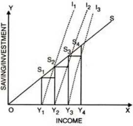
Fig. illustrates how different investment functions (I₁, I₂, I₃) interact with the fixed saving function (S). At each income level (Y₁, Y₂, Y₃, Y₄), the intersection of investment and saving determines equilibrium. Changes in investment expectations shift the equilibrium, emphasizing Harrod’s view that maintaining growth equilibrium is precarious and sensitive to investment behavior.
4. The Warranted Growth Rate
- Definition of warranted growth (Gw): The warranted growth rate is the rate of GDP growth at which entrepreneurs are fully satisfied with the prevailing economic conditions, so they have no incentive to change their investment behavior. In Harrod’s words, it’s the growth rate that “if achieved, will keep the economy moving steadily along a path of full capacity use.” Formally, it is the growth rate that keeps the capital-output ratio and the saving-investment equilibrium intact over time.
- We derived earlier that an equilibrium growth requires [latex]\frac{\Delta Y}{Y} = \frac{s}{v}[/latex]. This value [latex]\frac{s}{v}[/latex] is precisely the warranted rate of growth. Let’s denote it as Gw. Thus:
- [latex]G_{w} = \frac{s}{v}[/latex].
- For example, if s = 0.25 (25% of income saved) and v = 5 (₹5 of capital yields ₹1 of output), then [latex]G_{w} = \frac{0.25}{5} = 0.05[/latex], or 5% per year. At 5% annual growth, all the saving (25% of output) is exactly enough to equip the 5% increase in output with new capital (since output rising 5% requires a 5% rise in capital stock, and 5% of the initial output is 0.05 Y, times v=5 gives 0.25 Y of new capital, matching the saving).
- Entrepreneurs’ equilibrium: At Gw, businesses find their expectations met:
- If the economy grows at Gw, then actual investment equals planned investment. Firms have invested just the right amount: the new capital they install is exactly what’s needed to meet the growth in demand. There are no unintended inventory build-ups or shortages.
- Because of this, firms are content to keep investing at the same proportional rate. In other words, Gw is a self-replicating growth rate – if the economy manages to be on this growth path, it will tend to continue on it because all parties are satisfied (no one has a reason to change their saving or investment behavior).
- Harrod called this the “warranted” rate in the sense that it is warranted by the decisions of investors: it justifies or validates the prior investment decisions. It is sometimes also referred to as the “equilibrium growth rate” of the model, since it’s the only growth rate where the economy’s moving parts remain in consistent balance.
- Full capacity utilization: One hallmark of the warranted growth path is that capital (and by assumption, labor insofar as it was initially fully employed) is fully utilized without glut or shortage.
- At Gw, the capital-output ratio remains constant at v because capital and output grow in tandem. For instance, if the economy is growing at 5% in the above example, both output and the capital stock increase by 5%. The new capital added maintains the same ratio with the new output, implying no excess capacity.
- Additionally, all output produced finds demand. Since saving (which withdraws some income from consumption) is exactly translated into investment spending, total demand grows at the same rate as output supply. There is neither overproduction (which would cause unsold goods and idle capacity) nor underproduction (which would cause shortages and pressures to expand).
- Contrast with other growth rates: If the economy tries to grow at a rate different from Gw, these nice properties break down (leading to disequilibrium, covered in later sections). The warranted rate is essentially a knife-edge balance:
- At G < Gw (actual growth lower than warranted), the economy is not investing enough to absorb all savings, meaning not all capacity is utilized – this leads to falling utilization and other problems.
- At G > Gw (actual growth higher than warranted), investment is more than what current savings would support, leading to pressures on capacity (and potentially inflationary conditions or other imbalances).
- Thus, Gw is that unique growth rate that avoids these problems. It’s like the “just right” Goldilocks pace for the economy in this model – neither too slow to cause slack nor too fast to cause strain.
- Endogenous nature of warranted rate: Notably, Gw is determined by internal parameters of the model (s and v) rather than by external factors. In that sense, the warranted growth is endogenously determined in the Harrod model.
- This was a novel concept at the time: the long-run growth rate of the economy could be seen as something coming out of the saving behavior of households and the technology of production (capital requirements). It wasn’t guaranteed by some natural law; it depended on how people saved and how productively capital could turn those savings into output.
- In contrast, classical economists often thought the economy would gravitate to full employment growth based on supply-side factors. Harrod showed that even if supply factors (labor, etc.) allow a certain growth, the actual realized growth can be constrained by demand (through s and v), which yields this warranted rate.
- Warranted growth vs. actual policies: In practical terms, the concept of Gw implies that to achieve steady growth, a country may need to adjust its saving rate or capital efficiency.
- For example, if Indian policymakers in the 1960s observed that the warranted growth given existing s and v was only ~4%, but they desired higher growth, they would know that without changing those parameters the economy would face imbalances. This insight might push policies to increase the saving rate (through austerity or financial development to mobilize savings) or to improve the efficiency of investment (reduce v via better technology or capacity utilization).
- The warranted rate gives a target or benchmark: if actual growth is consistently below Gw, it signals under-investment or demand deficiency relative to capacity, whereas if it’s above, it signals an overheating relative to the economy’s saving capacity.
5. Actual Growth versus Warranted Growth: Disequilibrium Dynamics
- Actual growth rate (Ga): This is the realized rate of increase of output (GDP) in the economy. It is given by [latex]G_{a} = \frac{\Delta Y_{actual}}{Y}[/latex] for a given period. Actual growth depends on the actual level of investment that takes place and the resultant expansion of output.
- In the Harrod model, actual investment may or may not coincide with the amount needed to grow at Gw. If investors for some reason invest more or less than what the warranted rate calls for, the actual growth will differ from s/v.
- For example, suppose the warranted growth Gw for an economy is 6% (based on its s and v). If businesses become very optimistic and invest such that the economy’s output actually grows by 8% (Ga = 8%) this year, then Ga > Gw. Conversely, if pessimism leads to weak investment and output only grows 3%, then Ga < Gw.
- Disequilibrium and its immediate effects: When Ga deviates from Gw, the economy is thrown off the steady growth path. In practical terms, this means planned saving and planned investment were not equal:
- If Ga > Gw: The economy grew faster than the equilibrium rate. Typically this scenario implies that firms invested more than usual relative to current output (or consumers saved less than usual), resulting in demand outpacing the “normal” capacity growth. There will be signs of excess demand in the economy:
- Businesses find that their stocks of goods (inventories) might be running low because sales grew faster than expected. Machinery and factories are being utilized at above-normal capacity to meet the unexpected higher demand.
- Since actual investment was higher, the capital stock did increase more rapidly, but even so, output growth being above warranted means capacity is strained – the capital-output ratio v might temporarily drop (meaning output per unit of capital rose, often by working overtime or more shifts).
- In terms of saving-investment: ex ante, investors planned to invest more than what households planned to save. The imbalance (I > S planned) forced the economy into higher growth, which in turn might have been facilitated by unintended drops in inventories or drawing down unused capacity.
- If Ga < Gw: The economy grew more slowly than the equilibrium rate. This often means firms invested less than needed to maintain the warranted pace (or consumers saved more than investors wanted to invest). The result is excess supply and underutilized resources:
- Businesses accumulate unsold inventories because output (supply) exceeded demand growth. Factories and machines are not fully used; capacity lies idle because the increase in output was too small to absorb even the normal expansion of capacity.
- Here the capital-output ratio v may effectively rise above its normal level, as capital stock grew (even if modestly) while output lagged, leaving some capital underutilized.
- In saving-investment terms: ex ante, planned saving exceeded planned investment (S > I). The excess saving meant insufficient demand, causing output growth to falter until ex post saving fell back in line with lower investment.
- In either case, ex post saving will still equal ex post investment (since any surplus saving translates into unintended inventory investment, and any excess investment draws down inventories or financial assets). But the key is that the economy’s growth rate diverged from the steady-state path, leading to either slack or strain.
- If Ga > Gw: The economy grew faster than the equilibrium rate. Typically this scenario implies that firms invested more than usual relative to current output (or consumers saved less than usual), resulting in demand outpacing the “normal” capacity growth. There will be signs of excess demand in the economy:
- Short-run adjustment mechanisms: In a Keynesian view, when these imbalances occur, there are short-run pressures that push the economy further away from the warranted path:
- If demand exceeded expectations (Ga > Gw), firms seeing inventories depleted and strong sales will react by ramping up production and likely planning even more investment to expand capacity. This tends to sustain or even increase the growth momentum in the short run (a boom dynamic).
- If demand fell short (Ga < Gw), firms cut back production to prevent inventory build-up and become cautious on new investment. This can lead to an even slower growth or stagnation (a recessionary dynamic).
- Thus, an initial divergence of actual growth from the warranted rate doesn’t self-correct easily in this model; it tends to reinforce itself at least in the short term. There is an absence of an automatic stabilizer in Harrod’s framework to bring Ga back to Gw.
- Implication: the economy is on a ‘knife-edge’: The warranted growth path is delicately balanced. Any small perturbation – say a slightly higher investment one year boosting Ga above Gw – sets in motion forces that push the economy further from equilibrium rather than back toward it.
- We call the equilibrium “knife-edge” because maintaining Ga = Gw is precarious. A tiny shortfall or excess in aggregate demand leads to cumulative divergence (this concept will be further analyzed in the next section on instability).
- In real economies, there are other dampening factors (like price adjustments, changing interest rates, etc.), but under Harrod’s strict assumptions those are absent or ineffective. Therefore, once the actual growth departs from warranted, the model predicts growing instability unless something external intervenes.
- Example – a simple numerical illustration: Assume an economy where warranted growth Gw is 5%. Now imagine two scenarios:
- Boom deviation: Firms, expecting good times, invest such that GDP actually grows 7% this year (Ga = 7%). Now inventories drop and factories run hot. Encouraged, firms plan even more investment next year. Unless saving behavior somehow changes, next year could see even higher growth, say 8%, before maybe resource constraints like labor or inflationary pressures kick in. The initial 2% point positive gap led to a cumulative boom.
- Slump deviation: Alternatively, suppose businesses lose confidence and cut investment, yielding only 2% growth (Ga = 2%). Excess inventory piles up; seeing this, firms become pessimistic and may further cut capital spending. The economy could slip into near-zero growth or even contraction, a downward spiral triggered by the initial 3% point shortfall.
- These simplified scenarios illustrate Harrod’s point: steady 5% growth is not automatically restored; instead the economy either surges ahead or falls behind further if left unchecked.
- Transition: So far, we identified that any divergence between actual and warranted growth creates disequilibrium. Next, we examine in detail why this divergence tends to widen over time – Harrod’s famous instability or “knife-edge” condition – and how the model portrays the inherent difficulty of maintaining steady growth.
6. The Natural Growth Rate
- Definition of natural growth (Gn): The natural rate of growth is the maximum rate at which the economy can grow in the long run given the growth of factor supplies, primarily labor (and technology). It is the rate of output growth that maintains full employment of the labor force (and full utilization of other natural resources) over time.
- In a simple scenario with no technological progress, Gn is essentially equal to the growth rate of the labor force (population growth in the workforce). For example, if the labor force increases by 2% per year, the economy can naturally expand up to about 2% annually without creating unemployment, assuming capital can be provided.
- More generally, if we account for technological improvement (which raises labor productivity), the natural growth rate is the sum of labor force growth (n) and the rate of labor productivity growth (let’s call it p). So one can write: [latex]G_{n} = n + p[/latex]. If population of workers grows 1.5% a year and productivity (output per worker) grows ~1% via technical progress, then Gn ≈ 2.5% per year.
- Harrod described Gn as “the rate of advance which the increase of population and technological improvement allow.” It’s essentially the rate at which the economy’s capacity can expand from the supply side.
- Full employment growth requirement: If the economy grows at Gn, it is just absorbing all new entrants into the labor force (and utilizing any productivity gains) so that unemployment stays constant. Growing faster than Gn would typically require drawing down unemployment below normal or somehow increasing labor participation beyond usual levels (or an unsustainably high productivity jump). Growing slower than Gn means not all new workers find jobs, causing unemployment to rise.
- Thus, Gn can be thought of as the economy’s supply-determined ceiling for long-run growth under full employment. It is determined by demographic and technological factors.
- In India’s context, for example, during the 2000s the labor force was growing roughly ~2% per year. If productivity was improving by say 3% (through technology and better education, etc.), the natural growth rate might be around 5%. If India’s GDP grew consistently at 5%, it would more or less maintain stable employment levels given those supply-side conditions.
- No guarantee Gw = Gn: A crucial insight of Harrod’s model is that there is no inherent reason for the demand-determined warranted growth rate (Gw) to equal the supply-determined natural growth rate (Gn
- If [latex]G_{w} < G_{n}[/latex]: The warranted growth is below the natural rate. This means that even if the economy achieves the demand equilibrium (growing at Gw with full capacity utilization of capital), that growth might not be enough to absorb all the increase in labor supply. Over time, unemployment would tend to rise because the labor force is growing faster than jobs are created.
- In this scenario, the economy is essentially demand-constrained relative to its labor potential. There will be a chronic tendency for underemployment or surplus labor unless some mechanism boosts demand-side growth (like raising s/v or government intervention) or the labor supply growth slows down.
- Developing countries often found themselves in this bind: e.g., if a country’s population is growing at 3% annually but low savings yield a warranted growth of only, say, 2%, then even running the economy at Gw means 1% of the labor force (net) becomes unemployed each year. India in the mid-20th century, with high population growth and modest savings, faced such challenges – growth fell short of what was needed to fully employ the rapidly expanding workforce, contributing to persistent poverty and underemployment.
- If [latex]G_{w} > G_{n}[/latex]: The warranted growth is above the natural rate. In this case, the economy’s demand-driven expansion would, if achieved, outstrip the capacity permitted by labor growth (and technology). Trying to grow at Gw would encounter labor shortages and overheating long before that rate is sustained.
- Practically, if the economy tries to grow faster than Gn, unemployment falls below its “natural” level, and businesses start facing difficulty finding workers. This tends to trigger rising wages and possibly inflation. There may also be bottlenecks in other resources. These pressures can destabilize the growth – for instance, accelerating inflation might eventually choke off the boom or force policy tightening.
- In Harrod’s rigid model, wages and prices were assumed not to adjust easily to clear markets. So an economy with Gw > Gn faces a dilemma: there is more saving available than the growth limited by labor can utilize. One possible outcome is that actual growth will be forced down towards Gn due to labor shortage, but then not all savings can be invested (excess saving would cause a demand shortfall). The result could be a tendency toward recession unless offset by some other factor (like technological progress accelerating or a reduction in the saving rate).
- In either case, mismatch between Gw and Gn means that even the “balanced” warranted growth path is not a full-employment path (if Gw < Gn) or not a feasible path (if Gw > Gn) in the long run. The economy could suffer from either unemployment or inflationary pressure in trying to reconcile the two.
- If [latex]G_{w} < G_{n}[/latex]: The warranted growth is below the natural rate. This means that even if the economy achieves the demand equilibrium (growing at Gw with full capacity utilization of capital), that growth might not be enough to absorb all the increase in labor supply. Over time, unemployment would tend to rise because the labor force is growing faster than jobs are created.
- The Harrod problem of ‘secular’ gap: Harrod highlighted this as a fundamental long-run problem: an economy has to somehow adjust its saving rate or capital intensity (which determine Gw) to match the natural rate if it wants stable full-employment growth. Without such adjustment, policy makers might face a choice between chronic unemployment (if Gw < Gn) or inflationary booms (if Gw > Gn).
- In the context of economic planning, this meant that countries should aim to increase savings and investment enough to raise Gw to the level of Gn (so that the labor force is fully absorbed). Alternatively, measures to reduce population growth or dramatically improve technology (raising Gn) could help if Gw was persistently too low.
- Conversely, if an economy has a very high saving rate (and thus high Gw) but limited labor growth (low Gn), it might need to redirect some saving to other uses (or invest abroad, etc.) or encourage labor force growth (through immigration or higher participation) to avoid overheating.
- Natural rate in India’s case: In India today, for example, labor force growth has moderated (around 1–2% per year) and productivity growth can be 3–4% with technological and efficiency improvements, giving a Gn perhaps around 5–6%. If India’s policies manage to push the warranted growth (s/v) to, say, 7–8% (through high investment rates), there is a risk of facing labor constraints unless productivity rises faster or more workers enter the workforce. On the other hand, if the warranted rate were only 3% while Gn is 5%, India would see rising unemployment or an expanding low-productivity informal sector absorbing the surplus labor.
- This illustrates why balancing demand and supply side is critical. Harrod’s framework effectively requires that for a truly stable growth, one must aim for Gw = Gn – a condition that is not guaranteed by market forces alone.
7. Harrod’s “Knife-edge” Instability
- Dynamic instability of equilibrium: Harrod’s model famously implies that the steady growth equilibrium (where actual growth = warranted growth) is dynamically unstable. The metaphor of a “knife-edge” suggests that even a slight tilt or disturbance will cause the system to tip over to one side or the other – it won’t naturally return to balance.
- In a stable system (like in some later growth models), if growth strays from the equilibrium path, corrective forces push it back. But in Harrod’s system, deviations amplify themselves: once actual growth departs from Gw, the subsequent behavior of investors tends to push it further away.
- The reasoning, as we’ve seen: if actual demand is higher than expected, firms invest more and boost growth further (positive feedback), whereas if demand is lower, firms cut investment, depressing growth further (negative feedback spiral). There is no automatic moderating mechanism in the model’s assumptions.
- Centrifugal vs centripetal forces: Harrod described that around the equilibrium growth path, the forces are “centrifugal” – pushing the economy away – rather than “centripetal” (which would pull it back toward equilibrium).
- Imagine the warranted growth path as a narrow ridge or knife-edge. If the economy is exactly on that ridge, it can continue forward. But if it veers even slightly off (either to the left or right), it starts sliding down the slope away from the ridge. The farther it slides, the steeper the slope gets, carrying it further away.
- In mathematical terms, the equilibrium Ga = Gw is a unstable equilibrium point. Small perturbations do not die out; instead, they lead to increasing divergence of actual growth from warranted growth.
- Harrod’s own words: To capture this instability, Harrod wrote (paraphrased): “Only one growth rate is conducive to a steady state. Any departure from it produces forces that lead to further departure.” He noted that around the warranted rate “there are forces at work causing the system to depart further and further from the required line of advance.” This succinctly describes the knife-edge property.
- Consequences of instability: Because of this knife-edge character, Harrod’s model implies that an economy left to its own devices would likely not gravitate to steady growth. Instead, it might experience alternating bouts of too-fast growth (booms) and too-slow growth (recessions), rather than a smooth path.
- An economy could, for instance, accelerate into an investment boom overshooting full capacity, then crash when constraints or confidence issues arise – a cyclical outcome. Conversely, an underinvestment period can lead to stagnation and high unemployment until some external stimulus or adjustment occurs.
- In the pure model, without external interventions, one could imagine extreme outcomes: a persistent boom could lead to runaway inflation or resource exhaustion, whereas a persistent bust could lead to a depression. Real economies usually don’t go to infinity or zero in output – other mechanisms (like policy responses or the natural limits of capacity) intervene. But the model’s importance is highlighting that market forces alone, in this framework, do not ensure steady, balanced growth.
- Comparison to later models: This unstable outcome was a major criticism and puzzle. Later models (such as Solow’s) introduced factors like variable capital-labor ratios and price adjustments that act as stabilizing forces. In those models, if growth is above the long-run path, diminishing returns or rising factor prices slow it down; if below, unused capacity and lower capital per worker eventually spur faster growth – thus, equilibrium is restored.
- In Harrod’s world, none of these stabilizers operate automatically. The burden of stabilization would fall to external agents (like government policy) or sheer chance.
- This is why the Harrod-Domar model often was used to justify active government planning: since the market may not naturally maintain steady growth, planning and intervention could be needed to keep the economy on track.
- Visualizing the knife-edge: We can think of a simple graph: suppose we plot time on the x-axis and GDP on the y-axis. The warranted growth path would be a straight exponential curve (on a log scale, a straight line) representing constant growth Gw. If the actual path starts on that line but then deviates, the actual path will either curve upwards away (if a boom takes hold) or bend downwards (if a slowdown occurs). The gap between the actual path and the equilibrium path will widen over time without countervailing forces.
- Another way to picture it is to graph actual growth rate Ga against the deviation from equilibrium. In a stable system, if Ga is above target, next period Ga would fall, etc., represented by downward arrows bringing it back. In Harrod’s case, the arrows go outward – away from the center line – indicating divergence.
- While we won’t include a diagram here, the key point remains: maintaining Ga = Gw is like balancing a pencil on its tip; the smallest nudge and it falls.
- Cycle moderation (Hicks’ insight): Economist John Hicks in 1950 took Harrod’s instability framework and introduced the idea of upper and lower limits (a “ceiling” of full employment and a “floor” of minimum demand) to explain business cycles. In Hicks’ trade cycle model, the economy, if left unchecked, would try to boom infinitely (as Harrod suggests) but hits the ceiling when resources are fully employed, which stops further growth acceleration. Likewise, in a bust it would contract until it hits a floor (e.g., zero investment or some minimal consumption level), which prevents endless decline. The result is that Harrod’s explosive tendencies get reflected in oscillations – the economy cycles between boom and recession instead of diverging forever. This was an important refinement showing that adding non-linear constraints to Harrod’s linear model can yield more realistic cyclical behavior. It implies that while the equilibrium is still unstable, the real-world outcome might be recurring cycles rather than complete runaway or collapse.
- Implications for economic theory: Harrod’s knife-edge result was startling because it suggested that achieving steady growth at full employment might be inherently improbable in a laissez-faire economy. This provided a rationale for:
- Active fiscal and monetary policy: to counteract booms and slumps (Keynesian stabilization extended into the long run).
- Economic planning: to set investment targets such that actual growth stays close to warranted (many developing countries, including India in the 1950s-60s, took this lesson to heart, designing plans to try to harmonize investment with growth goals).
- Further theoretical development: It spurred economists like Robert Solow to seek models where growth could be stable. Solow’s 1956 model can be seen as a direct response, introducing flexibility and market mechanisms that naturally guide the economy toward a steady state growth (thereby avoiding the knife-edge).
- A nuanced view: Modern interpretations acknowledge that Harrod’s knife-edge is partly an artifact of the model’s rigid assumptions. In reality, some adjustments (inventory management, adaptive expectations, policy responses, etc.) do provide partial stability. Nonetheless, the insight is valuable: economies do exhibit momentum – booms can feed on themselves and downturns can worsen unless countered. Harrod’s model, in a stark way, captures this momentum effect in the absence of stabilizers.
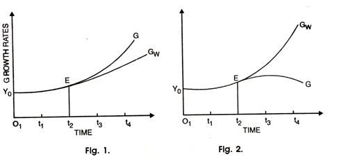
Fig. 1 shows actual growth (G) rising above warranted growth ([latex]G<sub>w</sub>[/latex]) leading to cumulative expansion.
Fig. 2 depicts actual growth falling below [latex]G<sub>w</sub>[/latex], resulting in stagnation. In both cases, point E (equilibrium) is unstable — once the economy deviates, it moves further away, highlighting the knife-edge nature of Harrod’s growth path.
8. Policy Implications in Harrod’s Framework
- Need for stabilization: Given the inherent instability (knife-edge) in Harrod’s model, government policy is seen as crucial to maintain the economy on a desirable growth path. In the absence of automatic market mechanisms to ensure steady growth at full employment, deliberate intervention can fill the gap.
- One key policy goal is to keep actual growth aligned with warranted growth (Ga ≈ Gw). This often means using counter-cyclical fiscal or monetary policies to dampen booms and boost slumps. For example, if the economy is growing too slowly (Ga < Gw) and unemployment is rising, the government can increase spending or cut taxes to stimulate demand, effectively raising actual growth toward the warranted level. Conversely, if the economy is overheating (Ga > Gw) with inflationary pressure, the government might reduce spending or the central bank might raise interest rates to cool off demand.
- Such stabilization policy extends Keynesian demand management into the long-run growth context. It’s not enough to achieve full employment once; the challenge is to maintain balanced growth year after year, which may require continual adjustments.
- Targeting the saving-investment balance: Since the warranted rate depends on s and v, policymakers can influence these to adjust Gw itself.
- Influencing the saving rate (s): Governments can adopt policies to change national saving. For instance, to raise s (if warranted growth needs to be higher), they might run budget surpluses, promote private saving through tax incentives, develop financial institutions (to mobilize household savings), or encourage corporate retained earnings. India’s early plans, for example, focused on increasing the savings rate via bank expansion and small-savings schemes to fund more investment. Conversely, if an economy’s saving is “too high” relative to useful investment opportunities (s making Gw exceed Gn), policies could encourage consumption (tax cuts, social safety nets) to lower s and thus avoid demand surplus.
- Influencing the capital-output ratio (v): While v is partly technological, policy can affect it by improving efficiency. Investment in better technology, infrastructure, or management practices can yield more output per unit of capital (lowering v). Education and skill development can also make labor more productive with the same capital. In development planning, reducing the ICOR (incremental capital-output ratio) is often a goal – meaning achieving more growth from each unit of investment. If v can be reduced, the same saving yields a higher Gw.
- Public investment: The government can directly inject investment into sectors to complement private investment. Public infrastructure projects, for example, not only utilize savings but can also lower costs for private sector (effectively reducing v economy-wide over time by raising productivity).
- Addressing the Gw vs Gn mismatch: If warranted growth is below natural growth (Gw < Gn), as is common in developing economies with rapid population growth but low savings, policy must strive to raise Gw or otherwise face rising unemployment.
- Development policy in such cases focuses on increasing investment (thus raising s or accessing foreign capital) to push the economy toward a higher growth trajectory. This was precisely the rationale behind India’s Second Five-Year Plan (1956–61) under Mahalanobis: to raise the investment rate in heavy industries so that long-term growth capacity (and thus warranted growth) would increase enough to absorb the growing labor force.
- Alternatively, if Gw is above Gn, policy might need to channel excess savings elsewhere or boost the labor force. One solution could be promoting exports or foreign investment outflows – effectively using the surplus saving to invest abroad (this was seen in some high-saving East Asian economies, which invested in foreign assets when domestic opportunities saturated). Another solution is to invest heavily in skill upgrades and technology to raise productivity (increase Gn). Immigration-friendly policy or increasing retirement age could also expand the labor force if needed.
- Planning and indicative targets: Harrod’s model, by quantifying the relation between investment and growth, provided a toolkit for planners:
- Governments often set growth targets (desired G) and then estimate required investment (as % of GDP) using the Harrod-Domar formula. For instance, if India targeted 7% growth and assumed an ICOR (v) of 4, planners would aim for an investment rate about 28% of GDP (since 0.07 = s/4 implies s ≈ 0.28). If domestic savings fell short of this, it signaled a “savings gap” to be filled either by foreign aid/borrowing or by policy measures to boost saving.
- This kind of planning was evident in India’s third and fourth Five-Year Plans where incremental capital-output ratios were used to estimate how much investment was needed to achieve the targeted GDP growth. Policies were then geared to mobilize that level of resources.
- Even today, institutions like NITI Aayog consider the investment-to-growth linkage: for example, to sustain ~8% growth, they evaluate whether domestic savings plus foreign capital can reach the required ~30+% of GDP investment.
- Counter-cyclical vs structural policies: It’s useful to distinguish two roles of government:
- Short-run stabilization: smoothening out deviations of actual growth from warranted (as discussed, via fiscal/monetary tweaks). This addresses cyclical instability.
- Long-run development strategy: adjusting the fundamentals (s and v) so that warranted growth is high enough and aligns with natural growth. This addresses structural issues. In practice, development policy (building institutions, encouraging investment in priority sectors, population policies) comes into play.
- Harrod’s framework underlines that both types of intervention can be important: managing year-to-year fluctuations and engineering longer-term growth capacity.
- Development strategies influenced: Development economists built on Harrod-Domar in formulating strategies: for instance, the “Big Push” theory (Rosenstein-Rodan) argued that a minimum critical level of investment (across multiple sectors) is needed to lift an economy out of a low-growth trap – essentially a practical prescription resonating with Harrod’s idea that insufficient investment leads to underutilization. Similarly, debates about balanced versus unbalanced growth hinged on how to allocate investment: Ragnar Nurkse’s balanced growth argument was that broad simultaneous investment in many sectors would create complementary demand and avoid bottlenecks (aligning with Harrod’s emphasis on demand sufficiency), whereas Albert Hirschman’s unbalanced growth strategy focused on investing in key sectors to stimulate growth via linkages, implicitly trusting that market forces would react and fill demand gaps in other sectors. Both views, in different ways, were responses to the fundamental challenge highlighted by Harrod – how to stimulate and sustain enough investment to utilize resources fully and grow rapidly.
- Limitations: While active policy is advocated by the model, it’s not without challenges:
- Incorrect assessment of v or over-ambitious investment drives can lead to inefficiencies (e.g., if funds are pushed into projects with low returns, v might actually rise, defeating the purpose).
- Political and social factors affect saving behavior and the feasibility of policies (for example, trying to raise the savings rate via austerity can hurt consumption and welfare in the short run).
- Additionally, external factors like trade demand or global financial conditions can upset domestic plans – something Harrod-Domar doesn’t explicitly cover but planners must consider.
- Nonetheless, the model’s implication that relying purely on market forces might not achieve optimal growth has been a cornerstone of post-war economic planning and policy discourse, especially in emerging economies.
9. The Harrod–Domar Model: Unifying Harrod’s and Domar’s Perspectives
- Evsey Domar’s contribution: While Harrod published in 1939, Evsey Domar independently developed a similar growth model in the mid-1940s (notably in a 1946 paper). Domar’s approach was motivated by the question: how much growth in output is needed to fully utilize new investment and prevent unemployment?
- Domar emphasized the dual effect of investment: (1) Investment increases aggregate demand (through spending on capital goods, which has a multiplier effect on income) and (2) Investment increases aggregate supply (by expanding productive capacity via new capital). For an economy to avoid idle capacity, these two effects must be in harmony.
- In Domar’s formulation, if σ is the productivity of capital (similar to 1/v in Harrod’s model), then an increment of investment ΔI adds σΔI to potential output in the next period. Meanwhile, the same ΔI, as spending, adds ΔI to demand initially (and more once multiplier effects are considered). Domar derived a condition that the growth rate of output must equal s/ v (essentially the same as Harrod’s) to ensure that the output created by new capacity is exactly matched by additional demand.
- Common equation: Both Harrod and Domar end up with the fundamental equilibrium growth formula:
- Growth rate = s / v = (Savings ratio) / (Capital–output ratio).
- Domar often expressed it in terms of the investment ratio (I/Y) and the capital productivity. Since in equilibrium I/Y = s (all saving is invested), one can see the overlap. In Domar’s terms, as long as output grows at that rate, the economy can absorb the increasing productive capacity without falling into unemployment or excess capacity.
- Thus, the Harrod-Domar model became a unified way to refer to this simple growth mechanism, highlighting that long-run growth depends on capital formation (investment) and the efficiency of capital use.
- Differences in emphasis: Despite the mathematical similarity, Harrod and Domar differed in emphasis:
- Harrod introduced distinct concepts (actual, warranted, natural growth rates) and was very concerned with the dynamic stability and the coordination problem over time. His analysis was more explicitly about the knife-edge instability and the condition for equilibrium.
- Domar’s analysis was a bit more centered on the insufficiency of demand: he framed the problem as achieving enough demand growth to utilize capacity. He did not delve as deeply into the question of instability, nor did he formalize a “natural” growth rate in his early work. Essentially, Domar assumed if labor and other resources were available, the key constraint was making sure demand kept up.
- Harrod’s model can be seen as more general in the sense of posing multiple potential gaps (demand vs capacity, and capacity vs labor), whereas Domar mainly tackled the demand vs capacity gap.
- Complementary insights: Together, the Harrod-Domar model provided a stark message: an economy must save and invest a significant portion of its income, and achieve sufficient efficiency in that investment, to grow steadily; otherwise, it will either stagnate or suffer from unused resources. In the post-WWII era, this message resonated with policymakers in developing countries.
- Harrod-Domar was used to justify large investment-push strategies. If growth was slow, one could diagnose either a low saving rate or a high capital-output ratio (perhaps due to technological backwardness or misallocation). The remedy would be to increase saving (domestic or via foreign aid) or improve investment efficiency.
- Domar himself was interested in avoiding depression: his work ties back to Keynes’s concern that inadequate demand (low investment) could lead to persistent unemployment. By formalizing the required growth of demand, Domar contributed to the understanding of secular stagnation risks.
- It’s worth mentioning that even before Harrod and Domar, economist Gustav Cassel (in the 1920s) had also written about a similar concept linking saving, investment and growth, but Harrod-Domar made it mainstream and embedded it in Keynesian macro thinking.
- Harrod-Domar in development planning: In economic development literature, one often sees references to the “Harrod-Domar formula.” For instance, development plans would say something like: “to achieve X% growth, given our capital-output ratio of Y, we need to attain a saving/investment rate of X×Y% of GDP.” This straightforward calculation comes directly from the model.
- Both Harrod and Domar gained recognition as co-creators of this foundational approach. Even though their original papers had nuanced differences, their names became linked in what essentially became the first generic growth model taught in development economics.
- The unified Harrod-Domar model was very popular with planners of under-developed countries in the 1950s–60s. It was simple and seemingly policy-actionable: increase the saving rate, and you can attain higher growth (given a technology parameter v). This led to a lot of emphasis on domestic resource mobilization and, where that was insufficient, on foreign aid to supplement investment – often called filling the “savings gap.”
- Limitations of the joint model: The unified Harrod-Domar model, while influential, carried the assumptions we have discussed (no factor substitution, fixed proportions, etc.) and therefore the same limitations. It doesn’t explain how technology changes or how factor prices adjust. These limitations set the stage for the next generation of growth theories (neoclassical and beyond).
- Nonetheless, as a first approximation, the Harrod-Domar model remains a handy tool. For example, if a policy analyst today asks, “Country A wants to grow at 10% a year, is that feasible given its investment rate of 20% of GDP?”, the Harrod-Domar lens quickly reveals that with a 20% investment rate, even with a very optimistic ICOR of 2, the maximum growth is 10%/ (assuming v = 5 gives 4% growth, or v = 2 which is unlikely). So 10% is out of reach without dramatically higher investment or efficiency. This kind of back-of-the-envelope analysis is a direct legacy of Harrod and Domar’s work.

This graph shows the savings function (S) and the total product of capital ([latex]TP<sub>K</sub>[/latex]) plotted against capital stock (K). Equilibrium occurs at point k₁, where savings equal the output generated by capital. Below k₁, savings (S₁) are insufficient to fully utilize capital, while above k₁, excess savings emerge. The diagram highlights Harrod’s concern with achieving balance between saving and capital productivity to maintain steady economic growth.
10. Harrod-Domar in Indian Economic Planning: Examples and Data
- Adoption in planning models: India was one of the earliest countries to integrate the Harrod-Domar logic into its economic planning. In the 1950s, as India launched its Five-Year Plans, economists like P.C. Mahalanobis (who crafted the Second Plan) explicitly used the concept of a fixed capital-output ratio and the required investment rate for target growth. The rationale was straightforward: to accelerate GDP growth, India needed to raise its rate of investment (since savings were scarce, this also implied seeking foreign aid to supplement domestic saving).
- In the First Five-Year Plan (1951–56), India’s gross domestic saving rate was very low (around 8–10% of national income). The plan targeted a modest 2.1% annual GDP growth, but thanks to good harvests, actual growth averaged about 3.6%. This was above target largely because agricultural output surged, not due to any major industrial investment push.
- By the Second Plan (1956–61), the goal was more ambitious industrial growth. Planners estimated the overall capital-output ratio for the economy to be about 3.5–4. They set a target growth rate of 4.5% per year. To achieve this, they calculated the required investment rate as roughly 4.5% × 4 ≈ 18% of GDP. Indeed, during the Second Plan period, India’s gross investment rate was raised to around 15–17% of GDP (with help from foreign aid and deficit financing). The actual growth achieved was about 4.3% annually – quite close to the target, validating the Harrod-Domar calculation to some extent.
- The “Hindu rate of growth” and ICOR: From the 1950s through the 1970s, India’s GDP growth averaged about 3.5% per year – a phenomenon jokingly dubbed the “Hindu rate of growth.” Harrod-Domar reasoning provides an insight into this prolonged sluggish growth:
- During that period, the domestic saving and investment rates in India hovered around 10–20% of GDP (rising gradually from the low teens in the 1950s to around 19–20% by the late 1970s). Meanwhile, the incremental capital-output ratio (ICOR, effectively v) observed was roughly 4 to 5 (meaning each 1% of GDP growth required 4-5% of GDP investment).
- Plugging those into the formula: with s ~ 0.15 and v ~ 4.5, the warranted growth Gw ≈ 0.15/4.5 = 0.033 or 3.3% per year. This is remarkably close to the actual average growth (~3.5%). It suggests that, on average, India was growing at about the rate predicted by its saving-investment capacity. The limitation was not mysterious – low savings constrained growth.
- This simple analysis supported the push for higher saving and investment. Indian policymakers consistently aimed to lift the investment rate. By the Fifth Five-Year Plan (1974–78), the target growth was 4.4% and with efforts to raise investment, actual growth marginally exceeded target at 4.8%. Still, high population growth meant per capita gains were small.
- Post-1991 acceleration: After economic liberalization in 1991, India’s growth trajectory changed significantly. One contributing factor, in Harrod-Domar terms, was the sharp rise in the saving and investment rates.
- In the 2000s, India’s gross investment rate rose to around 30% of GDP or higher (crossing 35% in some years around 2007). The ICOR in this period was estimated around 4. This would imply a potential growth rate Gw ≈ 30%/4 = 7.5% per year. Indeed, India recorded GDP growth averaging about 8% per year from 2003 to 2012, aligning well with the model’s prediction.
- For example, during the Eleventh Plan (2007–2012), the Planning Commission noted that to achieve ~9% GDP growth, an investment rate near 36–37% of GDP was required, assuming an ICOR of about 4. In reality, India’s investment was around 35–36% and growth averaged ~8.2%, slightly below target partly due to the global financial crisis. The shortfall can be interpreted as the effective ICOR being a bit higher or external demand weakening.
- These numbers show the continued relevance of the Harrod-Domar concept: policymakers still speak in terms of how much investment is needed for a desired growth. In 2019, when setting a goal to become a $\text{5 trillion economy, Indian policymakers discussed the need to sustain growth around 8-9\% and recognized that would likely require investment on the order of 38-40\% of GDP given prevailing efficiency levels.
- Nonetheless, the fundamental insight holds: to achieve sustained high growth, a country like India must maintain high levels of investment and strive to make that investment as efficient as possible. This is Harrod’s model in action – a testament to its enduring practical relevance.
- Sectoral ICOR and planning: Indian planners also understood that the capital-output ratio was not fixed universally – it differed by sector. Heavy industries had high v (lower output per capital initially) whereas services or agriculture might have lower v. The Mahalanobis strategy deliberately invested in heavy industry despite its high capital requirements, expecting long-term payoffs. This caused an initially high aggregate ICOR, meaning growth did not immediately jump proportionally to investment in the short run.
- Over time, as those heavy industries came online, they supplied machinery and inputs to other sectors, helping reduce bottlenecks. The hope was to reduce v in the long run by building domestic capacity (rather than relying on imports). In effect, the strategy was to temporarily tolerate a lower growth per unit of investment in exchange for future self-reliant growth.
- Critics like economist B.R. Shenoy had warned that overly ambitious investment via deficit financing could stoke inflation without commensurate growth, if the ICOR was underestimated. Indeed, in the Third Plan (1961–66) India aimed for 5–6\% growth but achieved barely 2.4\%, partly due to droughts and war, but also because investments didn’t translate to output as quickly as assumed, indicating an ICOR higher than expected.
- Savings gap and foreign aid: Indian planners also recognized the possibility of a savings-investment gap – when desired growth required more investment than available domestic savings. The Harrod-Domar framework in development economics gave rise to the concept of a “two-gap” problem: a savings gap and a foreign exchange gap. In India’s early decades, even when policy pushed domestic saving upward, limited foreign exchange to import capital goods was a bottleneck (foreign exchange gap). Models by economists like Chenery showed that foreign aid or external borrowing could help fill these gaps – essentially providing the additional investment and imports needed to reach growth targets. Indeed, India relied on external assistance in the 1950s and 60s to supplement domestic resources for planned investments.
- Plan outcomes in numbers: Over successive Five-Year Plans, one can see the Harrod-Domar logic play out:
- The Third Plan (1961–66) aimed for ~5.6\% growth with a sizable increase in investment, but a series of setbacks (poor monsoons, war, and perhaps an overestimate of how efficiently investment could convert to growth) led to only ~2.4\% actual growth. The ICOR turned out higher than expected. This taught planners to be cautious in assuming very low v (high efficiency).
- By the Seventh Plan (1985–90), India had raised the investment rate to ~24\% and targeted 5\% growth; it achieved about 6\% growth, partly due to better efficiency and some economic reforms improving productivity. The saving rate had increased significantly by then, showing progress.
- In the Eighth and Ninth Plans (1990s), and especially after liberalization, higher private savings and investment, along with foreign investment inflows, allowed growth rates above 6\%. The Tenth Plan (2002–2007) targeted 8\% and achieved an average of ~7.6\%. The Eleventh Plan (2007–2012) targeted 9\% and got ~8\% amidst a global recession – still an achievement attributable to investment peaking above one-third of GDP.
- In recent years, when investment in India slowed (post-2013), growth also decelerated to around 6–7\%, illustrating the model’s cautionary principle: if the investment rate falls and technology parameters remain similar, growth will inevitably slow. This remains a concern in current Indian planning – how to revive investment momentum to push growth back up.
- Global evidence: The importance of savings and investment for growth, as posited by Harrod-Domar, has been borne out in other countries as well. East Asian economies in the late 20th century (like South Korea, Taiwan, Singapore) achieved very high growth rates by mobilizing exceptional saving and investment levels. For example, South Korea’s investment often exceeded 30\% of GDP during its rapid industrialization, and it sustained growth rates of 7–10\% for decades (implying an ICOR around 3 to 4). China, starting in the 1980s, pushed its investment rate above 40\% of GDP and realized nearly 10\% average growth for 30+ years. These cases align with the Harrod-Domar principle that high investment (if used efficiently) yields high growth. Of course, these countries also benefited from improvements in education, technology, and governance – factors beyond the Harrod-Domar model – but the foundational role of capital accumulation was central.
- On the flip side, some economies with high investment did not sustain growth because of inefficiencies. The Soviet Union, for instance, invested heavily and initially saw fast growth mid-century, but by the 1970s its growth stagnated as the efficiency of investment plummeted (capital-output ratio worsened). This underlines that while quantity of investment matters (the focus of Harrod’s model), quality of investment (productivity of capital) is equally crucial – a nuance captured by the v term in the model. If v rises (meaning each unit of output requires more and more capital), then even very high saving may not translate to high growth.
11. Harrod’s Model vs Lewis’s Model vs Solow’s Model (Comparison)
The following table contrasts Harrod’s growth model with Arthur Lewis’s dual-sector development model and the Solow neoclassical growth model, highlighting key differences:
| Aspect | Harrod’s Growth Model (Keynesian) | Lewis’s Dual-Sector Model (Development) | Solow’s Neoclassical Growth Model |
|---|---|---|---|
| Nature of Model | Demand-driven growth model focusing on saving-investment dynamics in a single-sector economy. Emphasizes equilibrium growth rate and instability (macro perspective on sustained aggregate demand). | Structural change model with two sectors (traditional agriculture and modern industry). Emphasizes labor transfer from subsistence agriculture to industrial sector as the engine of growth (development economics focus). | Supply-side oriented growth model with a formal production function (capital and labor). Emphasizes capital accumulation, labor growth, and exogenous technological progress; forms the basis of modern long-run growth theory (neoclassical macro focus). |
| Key Assumptions | – Fixed capital-output ratio (no diminishing returns to capital).– Constant saving rate (s) exogenously given.– Labor not explicitly in production (assumed plentiful until “natural” limit is hit).– No automatic price/wage adjustment (Keynesian closure). | – Surplus labor in traditional sector (marginal productivity ~0) can be moved to modern sector without reducing agricultural output initially.– Modern sector has profit-driven investment; wages in industry remain at a near-subsistence level until surplus labor is absorbed.– Capital accumulation in the modern sector drives growth; traditional sector output grows little (labor productivity there stays low until labor exodus reaches a turning point). | – Diminishing returns to capital (capital productivity declines as K per worker rises).– Constant returns to scale in capital and labor combined (e.g., Cobb-Douglas production).– Saving rate exogenous, but flexible capital-labor ratio through substitution (firms adjust input mix based on factor prices).– Wages and interest rates adjust to clear labor and capital markets (full-employment assumption). |
| Primary Driver of Growth | Investment financed by savings. Growth depends on sufficient aggregate demand: the economy must invest enough (given v) to use all savings and expand output. The equilibrium growth is s/v (Harrod-Domar formula). Technological progress enters only via the “natural” rate (not explicitly modeled). | Capital investment in the modern (industrial) sector, fueled by reinvested profits. Growth occurs by absorbing cheap labor from the traditional sector, which keeps industrial wages low and profits (hence savings) high, allowing rapid capital accumulation. Structural transformation (shift of labor to higher productivity sector) is key. | Capital accumulation and technological progress. In the short run, higher saving/investment can raise growth (capital deepening), but due to diminishing returns, an economy converges to a steady-state income per capita. Long-run per capita growth comes from exogenous tech progress (since capital alone cannot drive perpetual growth). Population growth affects the level of income per person (more population dilutes capital per worker). |
| Role of Labor | Labor growth defines the natural limit (Gn). If population growth exceeds warranted growth, unemployment rises; if lower, labor shortages could arise. However, labor is not a direct input in the production function (output is a function of capital alone in the short run). Full employment of labor is not assured automatically. | Central to the model: assumes unlimited labor supply at a fixed subsistence wage in the traditional sector. The modern sector can expand employment without raising wages until the surplus labor is exhausted. Once that “Lewis turning point” is reached, wages begin to rise and the nature of growth changes (labor no longer essentially infinite). Thus, labor is the linchpin – abundant labor enables growth with constant real wage in early stages, and labor markets tighten only later. | Explicit factor of production. Labor (L) combines with capital (K) to produce output (Y = F(K,L)). The labor force grows at some exogenous rate (n). Full employment of labor is assumed in equilibrium (if there’s unemployment, wage reductions help restore it). An excessive labor force growth (high n) can reduce capital per worker and thus per capita income in the steady state. In Solow’s model, labor is subject to diminishing returns (if capital fixed), but an economy can always absorb more labor at a lower marginal product – no concept of surplus labor at zero marginal product. |
| Equilibrium & Stability | Steady growth at Gw (warranted) requires a delicate balance; it’s an unstable equilibrium (knife-edge). Left alone, the economy may not naturally achieve Gw, and any deviation tends to widen. No inherent mechanism ensures actual = warranted = natural growth. Thus, potential for cycles or persistent underemployment without policy intervention. | The model doesn’t focus on short-run stability/instability of growth rate; it is more about gradual change. As long as surplus labor exists, the modern sector can grow steadily by investment without wage pressures (implying a stable environment for industrial growth). When surplus labor is depleted, the economy transitions to a new state (wages rising) – at that point, growth may slow if not offset by productivity gains. Instability in the Harrod sense is not emphasized; the challenge is to make the structural transition smoothly. | The economy has a stable steady-state growth path. If the capital stock is above or below its steady-state level, automatic forces (diminishing returns and saving dynamics) push it toward equilibrium. The growth rate of output tends toward the natural rate (n + tech) in the long run. This stability means the model does not generate cycles internally – if actual growth deviates, say due to a shock, it will converge back to the steady state rather than diverge. Full employment growth at the natural rate is the norm in equilibrium (no knife-edge). |
| Outcomes & Implications | Highlights how a market economy might fail to use all resources: either chronic unemployment (if not enough investment) or demand-pull inflation (if too much). Underlines the importance of demand-side management and planning – government may need to stimulate investment or saving to achieve a desired growth target. Useful for setting investment requirements in planning (e.g., use ICOR to estimate needed investment). Lacks a long-run supply-side growth determinant (tech) – it’s a vehicle for analysis of potential instability more than a complete growth solution. | Explains the development process in labor-surplus economies: growth is initially fueled by moving labor from low-productivity rural work to high-productivity urban jobs without raising costs. This can lead to fast GDP growth and structural transformation. Once surplus labor is absorbed, the model implies a need to shift strategy (e.g., invest in human capital or innovation) to continue growth. Policy implications: invest in the modern sector, encourage labor mobility (rural to urban), and maintain high profit reinvestment rates. It also shows that wages and income distribution will eventually change as a result of development. | Explains income levels and growth across countries: economies with higher saving or lower population growth achieve higher steady-state income (more capital per worker), but long-run growth rates for all (in steady state) equal the exogenous rate of technological progress. Implication: boosting long-run growth requires technological advancement (innovation, education, R&D). Raising the saving rate accelerates growth temporarily (transitional) and raises the income level permanently, but doesn’t change the long-run growth rate of per capita output. Also, poorer countries can catch up (conditional convergence) if they have similar parameters (s, n, tech) – a phenomenon not present in Harrod or Lewis. Policy focus: create conditions for high investment and productivity gains (stable institutions, incentives for innovation, etc.), rather than worry about demand shortfalls (which are assumed resolved by price flexibility). |
| Relevance to India | Provided a framework for India’s early planning – e.g., setting investment requirements for targeted growth in the Five-Year Plans. Highlighted importance of increasing savings and capital formation. However, its assumptions of fixed coefficients sometimes led to overestimation of short-run growth (if investments were inefficient or delayed). India also encountered the model’s instability: periods of excess demand causing inflation, and periods of deficient demand causing idle capacity – leading to adoption of stabilization policies. The ICOR concept from Harrod-Domar is still used in policy discussions (e.g., to gauge efficiency of investment). | Reflects aspects of India’s trajectory: a large pool of underemployed rural labor has been gradually absorbed into higher productivity sectors (industry, services) over decades. In the early decades, industrial wages were relatively low, enabling profit-driven investment – somewhat akin to Lewis’s scenario. Even today, agriculture employs ~40-50\% of India’s workforce but produces <20\% of GDP – an indicator of surplus labor. Policies like Make in India, infrastructure push, etc., aim to shift surplus labor into productive jobs. The Lewis model reminds that this process can fuel growth without inflationary wage pressures until the surplus is reduced, at which point skill development and productivity growth must take over to sustain growth. | Useful for analyzing India’s long-run growth potential and the impact of factors like saving rates and population. Post-1991 reforms increased India’s productivity and effective use of capital, moving it closer to Solow-type conditions where high investment translates to higher income per capita. Solow’s emphasis on technology is relevant: India’s IT and services boom contributed to growth beyond what capital accumulation alone would predict. However, Solow’s full-employment assumption is often violated – India faces periodic unemployment and demand shortfalls (e.g., after 2008 or during COVID-19), where Harrod-type analysis (demand-side stimulus) is needed. Thus, India’s experience suggests a blend: in the long run, Solow’s supply factors drive growth, but in the short run, Harrodian demand management is crucial to reach that long-run path. |
12. Criticisms and Legacy of Harrod’s Model
- Key criticisms of assumptions: Economists have pointed out several unrealistic aspects of Harrod’s model:
- Fixed proportions & no factor substitution: In reality, if capital is relatively abundant and labor is scarce (or vice versa), firms can change techniques – use more labor-intensive methods or more capital-intensive ones. Harrod’s assumption of a fixed capital-output ratio ignores this flexibility. The Solow model later showed that allowing substitution leads to a more stable growth path (diminishing returns ensure convergence to equilibrium rather than explosive instability).
- No role for price adjustments: Harrod assumed wages and interest rates don’t adjust to clear labor and capital markets. In practice, if unemployment rises (warranted < natural), wage pressures might ease, making hiring labor cheaper, which can stimulate investment and eventually restore equilibrium. Similarly, if there’s excess demand, rising costs (prices, wages) can dampen it. By neglecting these feedbacks, Harrod likely overstated the knife-edge problem.
- Savings-investment dynamics: Treating the saving rate as exogenous overlooks that saving itself can be influenced by growth (e.g., higher income growth can generate higher saving). Also, investment decisions respond to interest rates and expectations in more complex ways than a constant s and naïve expectations. Harrod’s model in effect hard-coded a certain behavior that may not hold over time or in all contexts.
- Single-sector, closed economy: The model lumps the entire economy into one sector and ignores foreign trade or external capital flows. For many countries (like India), foreign aid or investment helped bridge the saving gap – something Harrod-Domar could accommodate only by altering s in the formula, not endogenously. It also doesn’t consider differences between sectors (which Lewis’s model does) or structural changes in production.
- Technological progress is exogenous: Harrod acknowledged technology via the natural growth rate, but the model doesn’t explain innovation. Solow’s critique was that long-run growth in per capita terms must come from technological progress – simply accumulating capital faces diminishing returns. Harrod’s model, with no diminishing returns, could imply indefinite growth from investment alone, which seems counter to empirical evidence (capital deepening eventually yields less boost).
- Empirical track record: Some aspects of Harrod’s predictions were not borne out in mature economies. For example, the extreme instability (“knife-edge”) is not fully observed – economies do experience booms and recessions, but they don’t typically explode or collapse entirely. The Great Moderation (period of reduced volatility in late 20th century) and the tendency of economies to converge (poorer countries catching up to richer, to a degree) are more consistent with the neoclassical view of stability via market adjustments.
- That said, Harrod’s concern about inadequate demand causing persistent unemployment did have historical validation (e.g., the Great Depression, or more recently Japan’s stagnation in the 1990s). His model captured the possibility of an economy operating below full capacity for extended periods – a concept later enriched by “underemployment equilibrium” ideas and which still informs Keynesian economics and policy (like debates on secular stagnation).
- Solow’s resolution: Robert Solow’s 1956 model directly addressed Harrod’s conundrums. By introducing a variable capital-output ratio (through a standard production function with diminishing returns), Solow showed that the economy has a unique stable steady-state growth path. In Solow’s model:
- The warranted growth rate adjusts to equal the natural rate in the long run because if capital accumulates too fast (raising K/L), the marginal product of capital falls, investment yields less growth, and the system self-corrects. If capital is too low, returns are high, spurring investment until balance is restored. Thus, full employment growth is achieved without knife-edge instability.
- Furthermore, Solow separated long-run growth into a component due to technological progress, explaining sustained per capita growth without ever-increasing investment ratios. In steady state, output grows at the natural rate (labor force growth + tech progress), and capital deepening stops – resolving Harrod’s warranted vs natural mismatch by effectively making warranted growth endogenous (it becomes the natural rate in equilibrium).
- Essentially, Solow preserved Harrod’s idea that saving and investment matter (they determine the steady-state income level and the speed of reaching it), but he eliminated the fragile dynamics by allowing flexibility and focusing on technology for ongoing growth. This made the model’s predictions more in line with observed economies (e.g., an economy can return to steady growth after a shock rather than spiraling away).
- Later developments: Harrod’s work paved the way for a rich field of growth theory:
- Endogenous growth models (Romer, AK models): In the 1980s and 90s, economists like Paul Romer revisited the idea of constant or increasing returns in aggregate (e.g., “AK models” where output = A·K, effectively linear in capital). Interestingly, these models have similarities to Harrod-Domar in that they can generate self-sustaining growth without exogenous tech progress and can exhibit multiple or path-dependent outcomes. However, they incorporate innovation, R&D, or human capital to justify non-diminishing returns, rather than assuming fixed coefficients. They also often avoid Harrod’s instability by different mechanisms (e.g., assuming forward-looking investment behavior, or government policies that guide the economy).
- Post-Keynesian and Harrodian growth theories: Some economists (Joan Robinson, Nicholas Kaldor, Luigi Pasinetti, etc.) built on Harrod’s demand-driven approach. For instance, Robinson introduced the concept of a “Golden Age” – a hypothetical situation where the economy’s warranted, actual, and natural growth rates coincide, resulting in smooth full-employment growth. She used this to analyze what conditions (in terms of wage flexibility or saving behavior) might permit a Harrodian economy to avoid instability. Kaldor, meanwhile, developed a model where he allowed the saving rate to differ between profits and wages, and argued that the distribution of income would adjust to ensure that saving equals investment in the long run (the so-called Kaldor-Pasinetti equilibrium). In essence, Kaldor was finding a mechanism (via income distribution changes) to achieve Harrod’s warranted growth endogenously. These contributions were complex, but they kept the focus on Harrod’s central question: how can an economy continually grow without disequilibrium?
- Thirlwall’s Law (balance-of-payments-constrained growth): In development macroeconomics, A.P. Thirlwall proposed that a country’s long-run growth can be constrained by external demand (exports) if domestic demand is sufficient but foreign exchange is lacking. This idea, while a trade-focused theory, resonates with Harrod’s demand-side perspective – emphasizing that aggregate demand (here, external) can cap growth below what internal capacity (natural rate) would allow. It extends the Harrod-Domar thinking to open economies, highlighting that in some cases the saving needed for investment is constrained by the ability to earn foreign exchange.
- Legacy and relevance: Despite its shortcomings, Harrod’s model left a lasting legacy:
- It was the first to formalize the possibility that insufficient demand (a mismatch between saving and investment plans) could derail long-run growth, not just short-run cycles. This influenced economic policy in the post-war era, justifying government involvement in investment and development planning (especially in newly independent nations trying to industrialize).
- Harrod’s concepts of warranted and natural growth introduced the notion that equilibrium growth is a knife-edge balance between capacity and demand, and also between the economy’s demand potential and labor supply. Later theory solved the “knife-edge” with different assumptions, but the tension between demand-side and supply-side factors in growth remains a central theme in macroeconomics.
- The Harrod-Domar model is still taught as a foundational stepping stone in growth economics. It’s appreciated for its simplicity and as a historical point of departure. Its basic formula (growth ≈ saving rate / capital-output ratio) remains an intuitively useful tool for back-of-envelope calculations and for highlighting the importance of capital formation in growth.
- For India and other developing countries, Harrod’s message about the need to raise savings and invest in productive capacity resonated strongly and in many ways laid the intellectual groundwork for decades of development policy. Many “growth acceleration” episodes in emerging economies (from East Asia’s boom to China’s rise) can be narrated in Harrod-Domar terms (high saving leading to high investment and growth, until diminishing returns or structural changes set in).
- Modern view: Today’s economists synthesize demand and supply factors in discussing growth. While Solow’s framework is the backbone for long-run supply-side growth analysis, many acknowledge that in the short-to-medium run, demand constraints (à la Harrod) can cause economies to underperform relative to their potential. This is evident in debates about “secular stagnation” in advanced economies – a situation where desired saving chronically exceeds desired investment, leading to sluggish growth unless corrected by policy (very much a Harrod-type concern). Central banks and governments deploy monetary and fiscal policies to address such gaps, implicitly validating Harrod’s point that managing aggregate demand is necessary even when focusing on long-run growth potential.
- Many low-income economies with meager savings have found themselves in a low-growth trap consistent with Harrod-Domar predictions – insufficient domestic saving means inadequate investment, and thus only marginal income gains, which in turn constrain future saving. Development strategies like foreign aid, external borrowing, or “big push” public investment are essentially attempts to break out of this trap by injecting capital from outside or from the state.
- In summary, Harrod’s Growth Model, though a product of its time and based on simplifying assumptions, remains theoretically significant as an early rigorous exploration of growth dynamics and practically relevant as a reminder that achieving sustained growth involves balancing the interplay of savings, investment, and the productive capacity of the economy.
Conclusion
Harrod’s Growth Model holds a distinctive place in economic theory and policy. Theoretically, it was a bold attempt to extend Keynesian thinking into the long run, positing that an economy’s growth rate is not automatic or self-correcting but hinges on the delicate balance of savings, investment, and capacity utilization. In doing so, Harrod introduced pivotal concepts – the warranted growth rate and the natural growth rate – that forced economists to recognize potential mismatches between the conditions for demand-side equilibrium and for full employment of resources. This was a seminal contribution: it highlighted that achieving steady, full-employment growth is a problem requiring analysis and perhaps conscious coordination, not something guaranteed by market forces.
Harrod’s formulation and its “knife-edge” implication spurred the development of modern growth theory. The evident tension in his model – an economy could chronically underperform or explode without adjustment mechanisms – motivated Robert Solow and others to seek more stable frameworks. In that sense, Harrod’s model was the catalyst for the entire neoclassical growth paradigm that dominates textbooks today. Even though the Solow model altered many of Harrod’s assumptions (allowing variable capital-output ratios and including technological progress explicitly), it was essentially solving the puzzle Harrod had set: how can economies grow with stability and full employment? The fact that Solow’s model answered this by incorporating factor substitutability and price adjustments underscores Harrod’s theoretical significance. His work delineated the problem that any satisfactory growth theory must address – the coordination of investment with both demand and supply factors over time.
From a practical standpoint, the Harrod-Domar model (as it became known in development economics) deeply influenced how policymakers, especially in countries like India, approached economic planning. In the early decades after independence, Indian planners faced the monumental task of lifting growth from colonial-era stagnation. Harrod-Domar provided a straightforward framework: to achieve a desired GDP growth rate, one must mobilize a certain proportion of national income for investment. This led to concrete investment targets in the Five-Year Plans and justified interventions to raise the saving rate, build capital stock, and channel funds into infrastructure and industry. The model’s emphasis on capital formation as the driver of growth validated the big infrastructure pushes – steel plants, dams, heavy industries – that characterized Indian development strategy in the 1950s and 1960s.
Importantly, Harrod’s model also carried warnings that were relevant to policy. It implied that merely accumulating capital without regard to balance could lead to issues – either idle capacity if demand lagged or inflationary pressure if demand outstripped capacity. Indian policymakers experienced both: periods of shortfall (as in the Third Plan when investments didn’t fully translate into growth) and periods of overheating (as in the late 1980s when demand had to be cooled to tame inflation). Harrod’s framework, thus, implicitly taught the need for complementary policies: alongside investing in capacity, one must manage aggregate demand and address structural bottlenecks (skills, technology, infrastructure) to get the most out of that investment.
In today’s context, India’s economy and policy toolkit have evolved, but the spirit of Harrod’s insights remains relevant. When Indian government think-tanks assess how to reach a }$5 trillion economy or sustain high growth, they invariably discuss required investment rates and incremental capital-output ratios – direct descendants of the Harrod-Domar formula. There is recognition that without boosting the investment rate (or improving investment efficiency), aspirations for higher growth will not materialize. Likewise, concerns about jobless growth link back to the idea of warranted vs. natural growth: if the economy grows below its natural pace, unemployment rises; if it tries to grow above without productivity gains, inflation and bottlenecks loom. Harrod’s model encapsulates this trade-off, reminding policymakers that sustainable growth requires equilibrium between what the demand side can support and what the supply side can deliver.
The broader significance of Harrod’s model today lies in its dual lesson. First, it underscores the importance of investment – in physical capital, human capital, and technology – as the fundamental engine of growth. This lesson has been internalized across the world; every rapidly growing economy has had high rates of investment, and every stagnating economy has struggled with insufficient or inefficient investment. Second, Harrod’s model is a cautionary tale about coordination and stability – market forces alone might not ensure that an economy’s savings are always optimally invested or that growth automatically uses all available labor. In advanced economies, this is seen in debates on secular stagnation and demand stimulus; in developing ones, it appears in discussions of output gaps and underemployment. The remedy invariably involves policy action, whether it’s monetary/fiscal stimulus to boost demand or structural reforms to improve efficiency – essentially echoing Harrod’s point that maintaining balanced growth often requires conscious effort.
In sum, Harrod’s Growth Model is theoretically significant as a pioneering framework that opened new vistas in growth theory, and it remains practically relevant, especially in contexts like Indian economic planning. It taught economists and policymakers to quantify growth requirements and to be vigilant about imbalances between investment and growth. While later models have refined our understanding and added realism (emphasizing technology, market adjustments, and human capital), Harrod’s core message endures: economic growth is not automatic – it results from deliberate investment effort and careful balancing of demand and supply forces. As India continues to pursue rapid, inclusive growth and as the world grapples with sustaining growth in the face of new challenges, the essence of Harrod’s insights – the need to plan, invest, and coordinate economic forces – remains as pertinent as ever. Harrod’s model, despite its age and simplifications, thus retains a profound legacy in guiding economic thinking, marrying theoretical rigor with actionable insight for achieving sustained development.
- Examine how the concepts of warranted and natural growth rates in Harrod’s model highlight structural issues in developing economies like India. (250 words)
- Compare Harrod’s growth model with the Lewis and Solow models in terms of their treatment of labor and implications for policy. (250 words)
- Discuss the relevance and limitations of Harrod’s knife-edge instability in the context of modern economic growth and planning. (250 words)

Responses